1. Empirical Checkerboard Copula

Oskar Laverny

2024-11-21

The empirical checkerboard copula is a model for copula defined by (Cuberos, Masiello, and Maume-Deschamps 2019). It provides a fast and easy way to model a copula in high-dimensional settings (more columns than rows in the dataset). It only requires one parameter, $m$, the so-called checkerboard parameter. In the first section of this vignette, we will set notations and define the model. The second section will discuss and demonstrate the implementation made in the package.

Definition of the empirical checkerboard copula

Suppose that we have a dataset with $n$ i.i.d observation of a $d$-dimentional copula (or pseudo-observations). Take the checkerboard parameter $m$ to be an integer dividing $n$.

Let’s consider the ensemble of multi-indexes $\mathcal{I} = \{\mathbf{i} = (i_1,..,i_d) \subset \{1,...,m \}^d\}$ which indexes the boxes :

$$B_{\mathbf{i}} = \left]\frac{\mathbf{i}-1}{m},\frac{\mathbf{i}}{m}\right]$$

partitioning the space $\mathbb{I}^d = [0,1]^d$.

Let now $\lambda$ be the dimension-unspecific Lebesgue measure on any power of $\mathbb{R}$, that is :

$$\forall d \in \mathbb{N}, \forall x,y \in \mathbb{R}^p, \lambda(\left[x,y\right]) = \prod\limits_{p=1}^{d} (y_i - x_i)$$

Let furthermore $\mu$ and $\hat{\mu}$ be respectively the true copula measure of the sample at hand and the classical Deheuvels empirical copula, that is :

• For $n$ i.i.d observation of the copula of dimension $d$, let $\forall i \in \{1,...,d\}, \, R_i^1,...,R_i^d$ be the marginal ranks for the variable $i$.
• $\forall x \in \mathcal{I}^d, \text{ let } \hat{\mu}([0,x]) = \frac{1}{n} \sum\limits_{k=1}^n \mathbb{1}_{R_1^k\le x_1,...,R_d^k\le x_d}$

We are now ready to define the checkerboard copula, $C$, and the empirical checkerboard copula, $\hat{C}$, by the following :

$$\forall x \in [0,1]^d, C(x) = \sum\limits_{\mathbf{i}\in\mathcal{I}} {m^d \mu(B_{\mathbf{i}}) \lambda([0,\mathbf{x}]\cap B_{\mathbf{i}})}$$

Where $m^d = \lambda(B_{\mathbf{i}})$.

This copula is a special form of patchwork copulas (see Durante) and some results are known about it : it is indeed a copula, it converges to the true copula as the mesh (size of boxes) goes to zero, etc..

This package gives a comprehensive implementation of the empirical counterpart of this copula, which has exactly the same expression except that $\mu$, the true copula of the sample, is replace by it’s Deheuvel approximation $\hat{\mu}$, that is :

$$\forall x \in [0,1]^d, \hat{C}(x) = \sum\limits_{\mathbf{i}\in\mathcal{I}} {m^d \hat{\mu}(B_{\mathbf{i}}) \lambda([0,\mathbf{x}]\cap B_{\mathbf{i}})}$$

A known result is that this is a copula if and only if $m$ divides $n$ (see cuberos). In this case, some theoretical assymptotics are avaliables.

The next section discuss the implementation.

Implementation

In this package, this empirical checkerboard copula is implemented in the cbCopula class. This class is a little more general as it allows for a vector $m = (m_1,...,m_d)$ instead of a single value. Each of the $m_i$’s must divide $n$ for this to be a proper copula. With the same train of thoughts as before, we have the following expression for this model :

$$\forall x \in [0,1]^d, \hat{C}(x) = \sum\limits_{\mathbf{i}\in\mathcal{I}} { \hat{\mu}(B_{\mathbf{i}}) \lambda([0,\mathbf{x}]\cap B_{\mathbf{i}})\prod\limits_{p=1}^{d}m_p}$$

You need to provide a dataset, defining $\hat{\mu}$, to construct the model. For the matter of this vignette, we will use the LifeCycleSavings dataset, which has following pairs dependencies plot :

set.seed(1)
data("LifeCycleSavings")
pseudo_data <- (apply(LifeCycleSavings,2,rank,ties.method="max")/(nrow(LifeCycleSavings)+1))

pairs(pseudo_data,lower.panel=NULL)

Pairs-plot of original peusdo-observation from the data

You can see that the variable 2 to 4 have dependencies, while the first and fifth variable seems to be (marginally) independent. The dataset having $n=50$ rows, we will pick a value of $m$ dividing $50$, e.g $m=5$, and use the function cbCopula to build our copula model. Since we are already providing the pseudo observations, we will set pseudo = TRUE. Providing a single value for the $m$ parameter will set all $m_i$’s equal to that value (the default is the proper checkerboard copula).

(cop <- cbCopula(x = pseudo_data,m = 5,pseudo = TRUE))
#> This is a cbCopula , with : 
#>    dim = 5 
#>    n = 50 
#>    m = 5 5 5 5 5 
#> The variables names are :  sr pop15 pop75 dpi ddpi

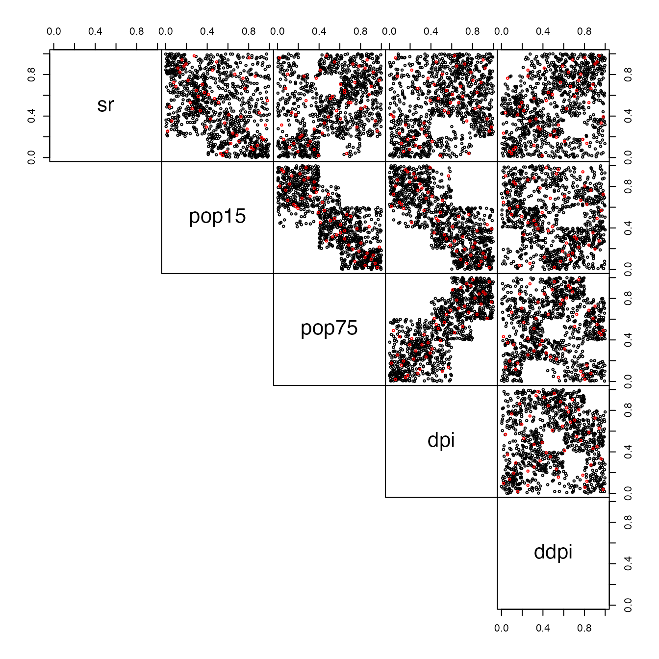
For the moment, only some methods exist for this copula. We can calculate it’s values via the pCopula method, or simulate from it via the rCopula method. the dCopula methods gives it’s density. Here is an example of simulation from this model :

simu <- rCopula(n = 1000,copula = cop)

pairs(rbind(simu,pseudo_data),
      col=c(rep("black",nrow(simu)),rep("red",nrow(pseudo_data))),
      gap=0,
      lower.panel=NULL,cex=0.5)

Pairs-plot of original peusdo-observation from the data (red) with simulated pseudo_observation (black)

About the value of $m$

The value of the checkerboard parameter $m$ condition heavily the copula itself. See the vignette about convex mixtures of m-randomized checkerboards for more details.

Cuberos, A., E. Masiello, and V. Maume-Deschamps. 2019. “Copulas Checker-Type Approximations: Application to Quantiles Estimation of Sums of Dependent Random Variables.” Communications in Statistics - Theory and Methods, March, 1–19.