3. Empirical Checkerboard Copula with known margins

Oskar Laverny

2024-12-26

The empirical checkerboard copula with known margins is a model for copula that uses priori information on a multidimensional margins to condition a checkerboard construction on the rest of the copula. This vignette describes the model in the first section, and then discuss current implementation in the second section

Empirical checkerboard copula with known margins

Preliminary notations

First of all, for a certain dimension of the data at hand $d$ and a certain checkerboard parameter $m$, let’s consider the ensemble of multi-indexes $\mathcal{I} = \{\mathbf{i} = (i_1,..,i_d) \subset \{1,...,m \}^d\}$ which indexes the boxes :

$$B_{\mathbf{i}} = \left]\frac{\mathbf{i}-1}{m},\frac{\mathbf{i}}{m}\right]$$

partitioning the space $\mathbb{I}^d = [0,1]^d$. Denote the set of thoose boxes by $\mathcal{B}_\mathcal{I} = \left\{B_{\mathbf{i}}, \mathbf{i} \in \mathcal{I}\right\}$. Furthermore, let’s choose $p$ dimensions that would be assigned to a known copula, by setting : $J \subset \{1,...,d\}, |J| = p$ and let’s define proper projections for the boxes :

$$B^J_{\mathbf{i}} = \{ \mathbf{x} \in [0,1]^p, x_j \in \left]\frac{i_j-1}{m},\frac{i_j}{m}\right] \forall j \in J \}$$

$$B^{-J}_{\mathbf{i}} = \{\mathbf{x} \in [0,1]^p, x_j \in \left]\frac{i_j-1}{m},\frac{i_j}{m}\right] \forall j \notin J \}$$

such that $B_{\mathbf{i}} = B^J_{\mathbf{i}} \times B^{-J}_{\mathbf{i}}$ for all $\mathbf{i} \in \mathcal{I}$. The tensor product is here understood taking dimensions of $\mathbb{I}^d = [0,1]^d$ in the right order such that $B^J_{\mathbf{i}}$ dimensions end up in place of dimensions indexed by $J$. Think of dimensions as re-ordered such that $J = \{1,...,p\}$.

Let now $\lambda$ be the dimension-unspecified Lebesgue measure on any power of $\mathbb{R}$, that is :

$$\forall d \in \mathbb{N}, \forall \mathbf{x},\mathbf{y} \in \mathbb{R}^p, \lambda(\left[\mathbf{x},\mathbf{y}\right]) = \prod\limits_{p=1}^{d} (y_i - x_i)$$

Let furthermore $\mu^J$ be a copula measure of dimension $p$, corresponding to the known multivariate margin associated to marginals in $J$. Let also $\mu$ and $\hat{\mu}$ be dimension-unspecific version of the true copula measure of the sample at hand and (respectively) the classical Deheuvels empirical copula, that is :

• For $n$ i.i.d observation of the copula of dimension $d$, let $\forall i \in \{1,...,d\}, \, R_i^1,...,R_i^d$ be the marginal ranks for the variable $i$.
• $\forall \mathbf{x} \in \mathcal{I}^d, \text{ let } \hat{\mu}([0,x]) = \frac{1}{n} \sum\limits_{k=1}^n \mathbb{1}_{R_1^k\le x_1,...,R_d^k\le x_d}$

We are now ready to define the empirical checkerboard copula with known margins.

Definition, estimation and simulation procedures

The empirical copula with known margins is the copula that correspond to the following simulation procedure.

• Simulate a sample from the known sub-copula $\mu^J$, of dimension $p$, through any avaliable method (depends on the known copula model). Let $B_{\mathbf{i}}^J$ be the (projected) box containing this sample.
• Sample one box $B_{\mathbf{i}}$ among all boxes with projection $B_{\mathbf{i}}^J$ with probability weights :
  • $\frac{\hat{\mu}(B_{\mathbf{i}})}{\hat{\mu}(B_{\mathbf{i}}^J)}$ if the projected box $B_{\mathbf{i}}^J$ contains one or more (empirical) data point, that is $\hat{\mu}(B_{\mathbf{i}}^J) \neq 0$
  • $\frac{\lambda(B_{\mathbf{i}})}{\lambda(B_{\mathbf{i}}^J)}$ otherwise.
• Simulate uniformly from $B_{\mathbf{i}}^{-J}$

This algorithm simulates first the known part of the model (dimensions in $J$), and then, conditionally, the checkerboard part, ensuring that the known copula is respected. The downside of this behavior is that the checkerboard part may have points outside standard checkerboard boxes, making this part of the copula less sparse than a true checkerboard. But is does become sparser as soon as the data fits the known margins. On the other hand, this algorithm allows for a lot of flexibility, mainly in the following points :

• The “grid” given by $\mathcal{B}_\mathcal{I}$ can be taken more arbitrarily than $m^d$ boxes of same volume, as soon as it’s a partition of $\mathbb{I}^d$.
• The known copula is not restricted at all and can be chose among all $p$-dimensionnal copulas.
• The estimation of the checkerboard part can be turn into a more flexible patchwork construction, by changing the independence copula for an other one inside the boxes. See Durante2013,Durante2015,Durante2015a

We are now going to define properly the measure associated to this simulation procedure, a.k.a the empirical checkerboard copula with known margins. Let $\nu$ be this measure and let $\mathbf{U}$ be a random vector drawn from it. Then $\forall \mathbf{x} \in \mathbb{I}^d$, following the above procedure, we have :

$$\nu([0,\mathbf{x}]) = \sum\limits_{{\mathbf{i}} \in \mathcal{I}} \mathbb{P}(\mathbf{U}^{-J} \in B_{\mathbf{i}}^{-J} \cap [0,\mathbf{x}^{-J}] | \mathbf{U}^{J} \in B_{\mathbf{i}}^{J} \cap [0,\mathbf{x}^{J}]) \mathbb{P}(\mathbf{U}^{J} \in B_{\mathbf{i}}^{J} \cap [0,\mathbf{x}^{J}])$$

While the unconditional term is easy to handle since it’s the measure associated with the known copula, $\mathbb{P}(\mathbf{U}^{J} \in B_{\mathbf{i}}^{J} \cap [0,\mathbf{x}^{J}]) = \mu^J(B_{\mathbf{i}}^{J} \cap [0,\mathbf{x}^{J}])$, the conditional term can be treated according to the algorithm : it will be $\frac{\lambda(B_{\mathbf{i}}^{-J} \cap [0,\mathbf{x}^{-J}])}{\lambda(B_{\mathbf{i}}^{-J})}$ inside a box chosen with probability conditional on $\hat{\mu}(B_{\mathbf{i}}^J) \neq 0$. We finally get the following definition :

The empirical checkerboard copula with parameter $m$ and with set of known margins $J$ following the measure $\mu^J$ is the copula corresponding to the measure $\nu$ given by :

$$\nu([0,x]) = \sum\limits_{{\mathbf{i}} \in \mathcal{I}} \mu^J(B_{\mathbf{i}}^{J} \cap [0,\mathbf{x}^{J}]) \frac{\lambda(B_{\mathbf{i}}^{-J} \cap [0,\mathbf{x}^{-J}])}{\lambda(B_{\mathbf{i}}^{-J})} \left[ \frac{\hat{\mu}(B_{\mathbf{i}})}{\hat{\mu}(B_{\mathbf{i}}^J)} \mathbb{1}_{\hat{\mu}(B_{\mathbf{i}}^J) \neq 0} + \frac{\lambda(B_{\mathbf{i}})}{\lambda(B_{\mathbf{i}}^J)} \mathbb{1}_{\hat{\mu}(B_{\mathbf{i}}^J) = 0} \right]$$

The next section will discuss the current implementation of this copula;

Current implementation

The package implements the empirical checkerboard copula with known margins through the cbkmCopula class. The constructor of the class takes several arguments :

• x, the pseudo_data.
• m=nrow(x), repesenting the checkerboard parameter
• pseudo=FALSE, is the pseudo_data already given in a pseudo_observation form ?
• margins_numbers=NULL, the margins index that are associated to the known copula, formerly noted $J$
• known_cop=NULL, the known copula to be applied to thoose margins : a copula object of right dimension.

for example, let’s take the LifeCycleSavings data :

set.seed(1)
data("LifeCycleSavings")
dataset <- (apply(LifeCycleSavings,2,rank,ties.method="max")/(nrow(LifeCycleSavings)+1))
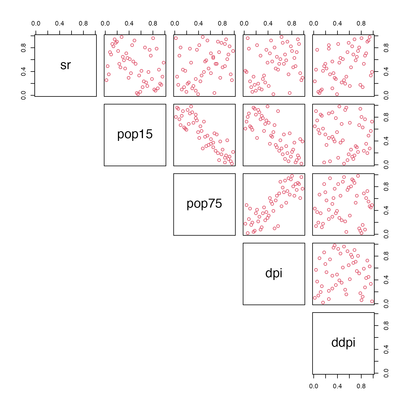
pairs(dataset,col="2",lower.panel=NULL)

Pairs-plot of original peusdo-observations

let’s now estimate a checkerboard copula on margins 2 and 3 with a precise $m=25$, and consider it to be known.

  known_margins <- c(2,3)
  known_copula <- cbCopula(x = dataset[,known_margins],m = 25,pseudo = TRUE)

Then we can construct the ECBC with this known margin :

  (cop <- cbkmCopula(x = dataset,m = 5,pseudo = TRUE,margins_numbers = known_margins,known_cop = known_copula))
#> This is a cbkmCopula , with : 
#>    dim = 5 
#>    n = 50 
#>    m = 5 5 5 5 5 
#> The variables names are :  sr pop15 pop75 dpi ddpi 
#> The variables  2 3  have a known copula  given by :
#>  This is a cbCopula , with : 
#>     dim = 2 
#>     n = 50 
#>     m = 25 25 
#>  The variables names are :  pop15 pop75

We can then simulate from it :

  simu <- rCopula(1000,cop)
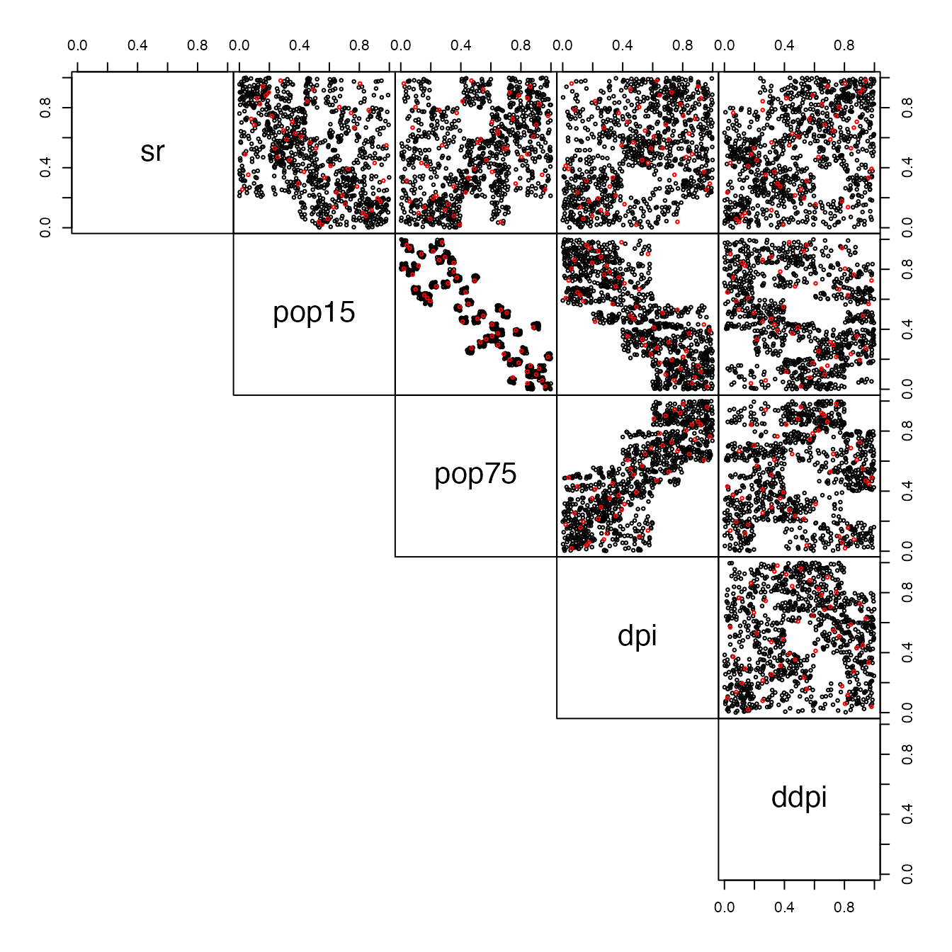
  pairs(rbind(simu,dataset),col=c(rep("black",nrow(simu)),rep("red",nrow(dataset))),gap=0,lower.panel = NULL,cex=0.5)

Pairs-plot of the original data (red) and simulated data from a good model (black)

You can see that the known margins were respected, which is the whole point of this model. Let now see an example with a clearly wrongly-specified copula for the known margins :

  bad_known_copula <- cbCopula(x = dataset[,known_margins],m = 2,pseudo = TRUE)
  cop <- cbkmCopula(x = dataset,m = 5,pseudo = TRUE,margins_numbers = known_margins,known_cop = bad_known_copula)

  simu <- rCopula(1000,cop)
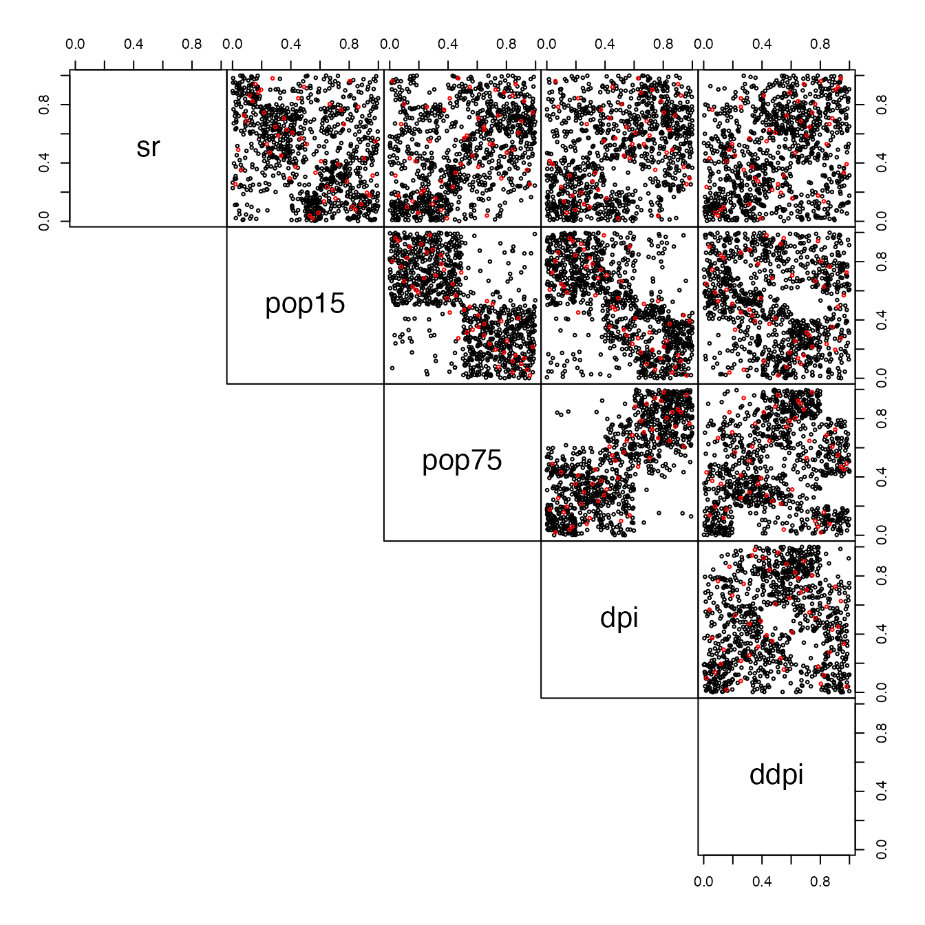
  pairs(rbind(simu,dataset),col=c(rep("black",nrow(simu)),rep("red",nrow(dataset))),gap=0,lower.panel = NULL,cex=0.5)

Pairs-plot of the original data (red) and simulated data from a wrong model (black)

This example shows the sensitivity of the estimation on other parts of the model to the good behavior of the prior estimate. The conditioning did suffer for the dependences inside the known multidimensional margin but also for dependencies involving one of the variables from thoose known margins. But the checkerboard construction for the other part of the copula was not harmed.

What now if the 2 parts are clearly independent ?

  true_copula1 <- known_copula
  true_copula2 <- bad_known_copula

  dataset <- cbind(rCopula(1000,true_copula1),rCopula(1000,true_copula2))
  colnames(dataset) <- c("u","v","w","x")
  pairs(dataset,lower.panel=NULL,cex=0.5)

Pairs-plot of the original data with independance

  cop <- cbkmCopula(x = dataset,m = 5,pseudo = TRUE,margins_numbers = c(1,2),known_cop = true_copula1)
  simu <- rCopula(500,cop)
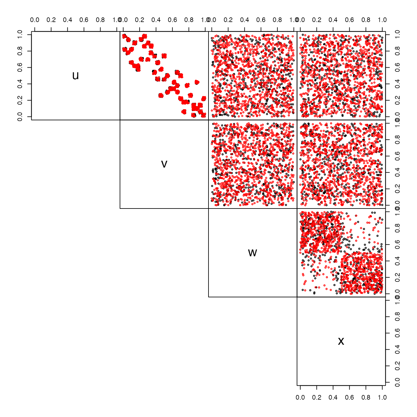
  pairs(rbind(simu,dataset),col=c(rep("black",nrow(simu)),rep("red",nrow(dataset))),gap=0,lower.panel = NULL,cex=0.5)

Pairs-plot of the original data (red) and simulated data (black) – Independance case

This fit is quite good.