2. The Copula Recursive Tree
2025-01-30
Source:vignettes/vignette02_cort_clayton.Rmd
vignette02_cort_clayton.RmdIntroduction
In this vignette, we will use the Cort algorithm to fit a copula on a given simulated dataset based on clayton copula simulations. We will show how the algorithm can be used to produce a bona-fide copula, and describe some of the parameters.
Dataset
First, let’s create and plot the dataset we will work with. For that,
we’ll use the gamma frailty model for the Clayton copula (but it’ll work
for any other completely monotonous archimedean generator), as it is
done in the copula package, see there.
The following code is directly taken from the previous link, from the
copula package :
psi <- function(t,alpha) (1 + sign(alpha)*t) ^ (-1/alpha) # generator
rClayton <- function(n,dim,alpha){
  val <- matrix(runif(n * dim), nrow = n)
  gam <- rgamma(n, shape = 1/alpha, rate = 1)
  gam <- matrix(gam, nrow = n, ncol = dim)
  psi(- log(val) / gam,alpha)
}
The following code simulates a dataset and then visualise it :
set.seed(12)
n = 200 # taken small to reduce runtime of the vignette.
d = 4
n_trees = 5 # taken small to reduce runtime of the vignette.
number_max_dim_forest = 2 # taken small to reduce runtime of the vignette.

data <- matrix(nrow=n,ncol=d)
data[,c(1,4,3)] = rClayton(n=n,dim=d-1,alpha=7)
data[,2] = runif(n)
data[,3] <- 1 - data[,3]

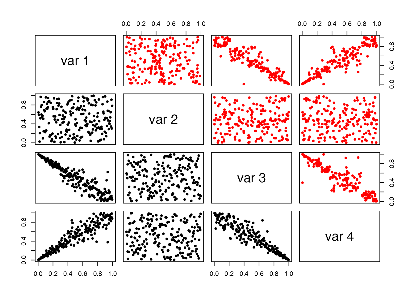
pairs(data,cex=0.6)
We can clearly see that the second marginal is independent form the rest. In the following we will use this package to fit this dependence structure.
Fitting the Cort copula
Now that we have a dataset, we can run the Cort algorithm on it. In
the implementation proposed here, this is done via the
cort::Cort() function, passing first the dataset, and then
various parameters. See ?Cort for a detailed list of
parameters. Note that the verbosity level is quite progressive: We will
here put it on 4 to see the splitting decisions that the algorithm is
making.
set.seed(12)
(model = Cort(data,verbose_lvl = 1))
#> Splitting...
#>
#>      1 leaves to split...
#>      7 leaves to split...
#>      14 leaves to split...
#>      9 leaves to split...
#>      6 leaves to split...
#>      2 leaves to split...
#>      4 leaves to split...
#>      7 leaves to split...
#>      5 leaves to split...
#>      11 leaves to split...
#>      19 leaves to split...
#>      14 leaves to split...
#> Enforcing constraints...
#> Done !
#> Cort copula model: 200x4-dataset and 418 leaves.
Looking at the top of the output, we see that the first thing the
algorithm did was removing the second dimension due to the independence
test. Now that the copula is fitted, we have access to numerous of it’s
methods. Two plotting functions are exported with this model, the
pairs function is implemented at a very low level in the
class hierarchy and hence is working with almost all copulas of this
package, but the plot function is only implemented for
Cort.
pairs(model)
Pairs-plot of original data (in black, bottom-left corner) versus a simulation from the model (in red, top-right corner)
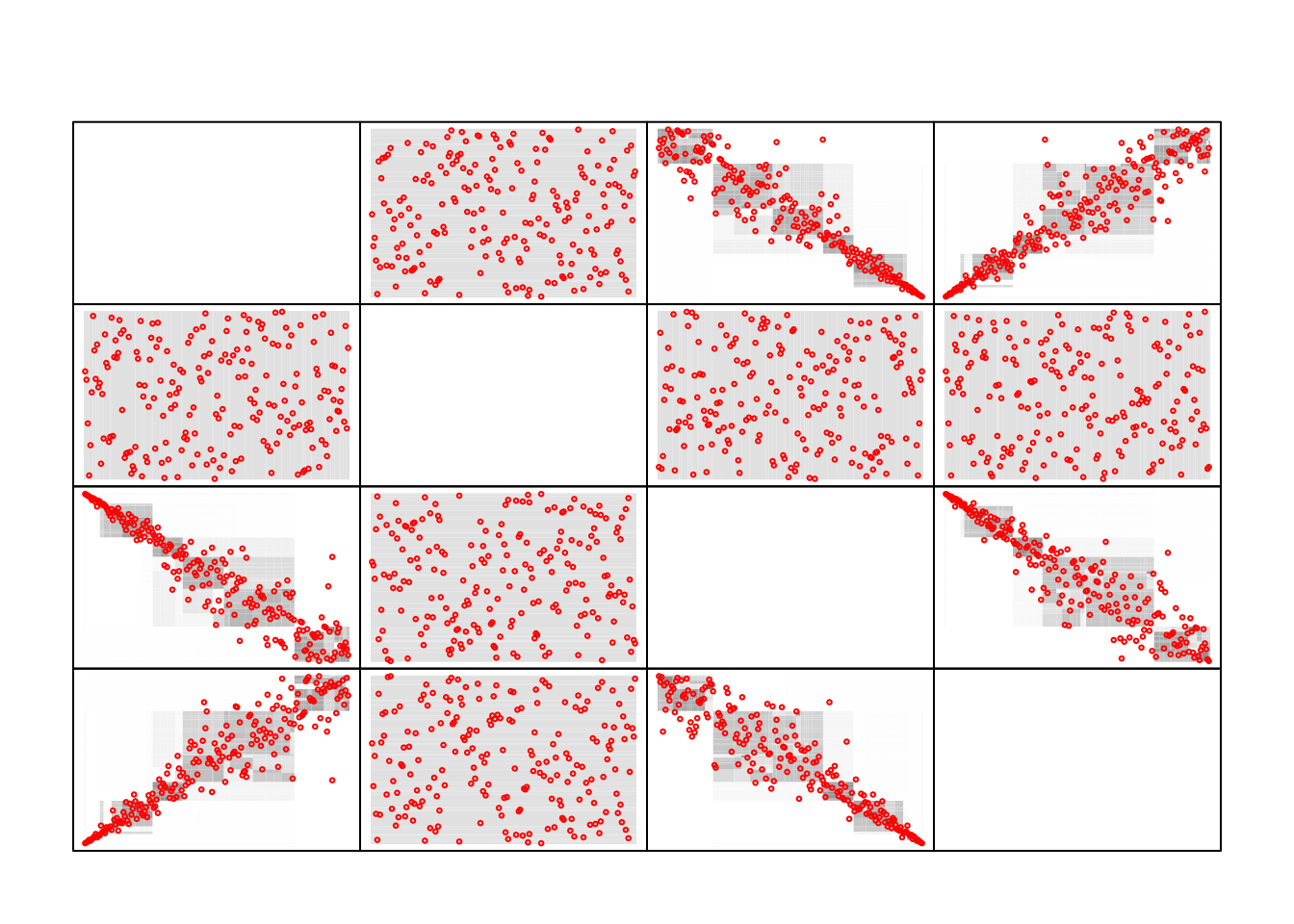
plot(model)
Gray boxes representing 2-d projections of the fitted density. In red, the imputed data points.
We see that there are some noise with point were there should not be.
A bagged version of the model is accessible via the
CortForest class, and might be able to correct these
problems.