Empirical models

Pseudo-observations

Through the statistical process leading to the estimation of copulas, one usually observes the data and information on the marginals scale and not on the copula scale. This discrepancy between the observed information and the modeled distribution must be taken into account. A key concept is that of pseudo-observations.

Definition: Pseudo-observations

If $\mathit{x}\in {\mathbb{R}}^{N\times d}$ is an $N$-sample of a $d$-variate real-valued random vector $\mathit{X}$, then the pseudo-observations are the normalized ranks of the marginals of $\mathit{x}$, defined as:

$$\mathit{u}\in [0,1{]}^{N\times d}:u_{i,j}=\frac{\mathrm{Rank}(x_{i,j},{\mathit{x}}_{\cdot ,j})}{N+1}=\frac{1}{N+1}\sum _{k=1}^N{\mathbb{1}}_{x_{k,j}\le x_{i,j}},$$

where $\mathrm{Rank}(y,\mathit{x})=\sum _{x_i\in \mathit{x}}{\mathbb{1}}_{x_i\le y}$.

In Copulas.jl, we provide a function pseudos that implement this transformation directly.

Copulas.pseudos Function

pseudos(sample)

Compute the pseudo-observations of a multivariate sample. Note that the sample has to be given in wide format (d,n), where d is the dimension and n the number of observations.

Warning: the order used is ordinal ranking like https://en.wikipedia.org/wiki/Ranking#Ordinal_ranking_.28.221234.22_ranking.29, see StatsBase.ordinalrank for the ordering we use. If you want more flexibility, checkout NormalizeQuantiles.sampleranks.

source

Deheuvel's empirical copula

From these pseudo-observations, an empirical copula is defined and anlysed in [58] as follows:

Definition: Deheuvel's empirical copula

The empirical distribution function of the normalized ranks,

$${\hat{C}}_N(\mathit{u})=\frac{1}{N}\sum _{i=1}^N{\mathbb{1}}_{{\mathit{u}}_i\le \mathit{u}},$$

is called the empirical copula function.

Theorem: Exhaustivity and consistency

$${\hat{C}}_N$$

is an exhaustive estimator of $C$, and moreover for any normalizing constants $\{{\varphi }_N,N\in \mathbb{N}\}$ such that $\underset{N\to \mathrm{\infty }}{lim}{\varphi }_N\sqrt{N^{-1}\ln \ln N}=0$,

$$\underset{N\to \mathrm{\infty }}{lim}{\varphi }_N\underset{\mathit{u}\in [0,1{]}^d}{sup}|{\hat{C}}_N(\mathit{u})-C(\mathit{u})|=0\text{ a.s.}$$

$${\hat{C}}_N$$

then converges (weakly) to $C$, the true copula of the random vector $\mathit{X}$, when the number of observations $N$ goes to infinity.

Info: The empirical copula is not a true copula

Despite its name, ${\hat{C}}_N$ is not a copula since it does not have uniform marginals. Be careful.

In the package, this copula is implemented as the EmpiricalCopula:

Copulas.EmpiricalCopula Type

EmpiricalCopula{d, MT}

Fields:

• u::MT — pseudo-observation matrix of size (d, N).

Constructor

EmpiricalCopula(u; pseudo_values=true)

The empirical copula in dimension $d$ is defined from a matrix of pseudo-observations $\mathbf{u}=(u_{i,j}{)}_{1\le i\le d,1\le j\le N}$ with entries in $[0,1]$. Its distribution function is

$$C(\mathbf{x})=\frac{1}{N}\sum _{j=1}^N{\mathbf{1}}_{\{{\mathbf{u}}_{\cdot ,j}\le \mathbf{x}\}},$$

where the inequality is componentwise. If pseudo_values=false, the constructor first ranks the raw data into pseudo-observations; otherwise it assumes u already contains pseudo-observations in $[0,1]$.

Notes:

• This is an empirical object based on pseudo-observations; it is not necessarily a true copula for finite $N$ but is widely used for nonparametric inference.

• Supports cdf, logpdf at observed points, random sampling, and subsetting.

References:

• [3] Nelsen, Roger B. An introduction to copulas. Springer, 2006.

source

Info: Conditionals and distortions

• Distortions: available via the generic implementation (partial-derivative ratios). For the empirical copula, derivatives are stepwise; interpret results carefully near sample jumps.

• Conditional copulas: available via the generic implementation. No specialized fast path is provided.

Visual: empirical copula from pseudo-observations

using Copulas, Distributions, Plots
# generate data with known dependence, then compute pseudo-observations
X = SklarDist(ClaytonCopula(2, 1.2), (Normal(), Beta(1, 4)))
x = rand(X, 1000)
Ĉ = EmpiricalCopula(x, pseudo_values=false)
plot(plot(X.C), plot(Ĉ); layout=(1,2))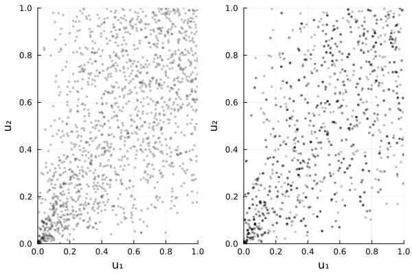

Beta copula

The empirical copula function is not a copula. An easy way to fix this problem is to smooth out the marginals with beta distribution functions. The Beta copula is thus defined and analysed in [59] as follows:

Definition: Definition (Beta Copula):

Denoting $F_{n,r}(x)=\sum _{s=r}^n(\genfrac{}{}{0ex}{}{n}{s})x^s(1-x{)}^{n-s}$ as the distribution function of a $\mathrm{Beta}(r,n+1-r)$ random variable, the function

$${\hat{C}}_N^{\beta }:\mathit{x}\mapsto \frac{1}{N}\sum _{i=1}^N\prod _{j=1}^d{F}_{n,(N+1)u_{i,j}}(x_j)$$

is a genuine copula, called the Beta copula.

Property: Proximity of $\hat{C}_N$ and $\hat{C}_N^\beta$

$$\underset{\mathit{u}\in [0,1{]}^d}{sup}|{\hat{C}}_N(\mathit{u})-{\hat{C}}_N^{\beta }(\mathit{u})|\le d(\sqrt{\frac{\ln n}{n}}+\sqrt{\frac{1}{n}}+\frac{1}{n})$$

In the package, this copula is implemented as BetaCopula:

Copulas.BetaCopula Type

BetaCopula{d, MT}

Fields:

• ranks::MT - ranks matrix (d × n), each row contains integers 1..n

Constructor

BetaCopula(u)

The empirical beta copula in dimension $d$ is defined as

$$C_n^{\beta }(u)=\frac{1}{n}\sum _{i=1}^n\prod _{j=1}^d{F}_{n,R_{ij}}(u_j),$$

where $R_{ij}$ is the rank of observation $i$ in margin $j$, and $U\sim Beta(r,n+1-r)$.

Notes:

• This is always a valid copula for any finite sample size n.

• Supports cdf, logpdf at observed points and random sampling.

References:

• [60] Segers, J., Sibuya, M., & Tsukahara, H. (2017). The empirical beta copula. Journal of Multivariate Analysis, 155, 35-51.

source

Info: Conditionals and distortions

• Distortions: specialized fast path returning a MixtureModel of Beta components for efficient evaluation and sampling.

• Conditional copulas: available via the generic implementation (no dedicated fast path).

Performance notes

• Construction is O(d·n) after pseudo-observations are computed. Evaluation at a point uses O(d·n) basis lookups; consider subsampling for very large n.

Bernstein Copula

Bernstein copula are simply another smoothing of the empirical copula using Bernstein polynomials.

Mathematically, given a base copula $C$ and degrees $\mathit{m}=(m_1,\dots ,m_d)$, the (cdf) Bernstein copula is

$$B_{\mathit{m}}(C)(\mathit{u})=\sum _{s_1=0}^{m_1}\cdots \sum _{s_d=0}^{m_d}C(\frac{s_1}{m_1},\dots ,\frac{s_d}{m_d})\prod _{j=1}^d(\genfrac{}{}{0ex}{}{m_j}{s_j})u_j^{s_j}(1-u_j{)}^{m_j-s_j}.$$

It is a multivariate Bernstein polynomial approximation of $C$ on the uniform grid. Larger $m_j$ increase smoothness and accuracy at higher computational cost.

In the package, this copula is implemented as BernsteinCopula:

Copulas.BernsteinCopula Type

BernsteinCopula{d}

Fields:

• m::NTuple{d,Int} - polynomial degrees (smoothing parameters)

• weights::Array{Float64, d} - precomputed grid of box measures

Constructor

BernsteinCopula(C; m=10)
BernsteinCopula(data; m=10)

The Bernstein copula in dimension $d$ is defined as

$B_m(C)(u)=\sum _{s_1=0}^{m_1}\cdots \sum _{s_d=0}^{m_d}C(\frac{s_1}{m_1},\dots ,\frac{s_d}{m_d})\prod _{j=1}^d(\genfrac{}{}{0ex}{}{m_j}{s_j})u_j^{s_j}(1-u_j{)}^{m_j-s_j}.$

It is a polynomial approximation of the base copula $C$ using the multivariate Bernstein operator.

Implementation notes:

• The grid of box measures (weights) is fully precomputed and stored as an $n$-dimensional array at construction. This enables fast evaluation of the copula and its density, but can be memory-intensive for large $d$ or $m$.

• The choice of m controls the smoothness of the approximation: larger m yields finer approximation but exponentially increases memory and computation cost ($\prod _j{m}_j$ boxes).

• For high dimensions or large $m$, memory usage may become prohibitive; see documentation for scaling behavior.

• If $C$ is an EmpiricalCopula, the constructor produces the empirical Bernstein copula, a smoothed version of the empirical copula.

• Supports cdf, logpdf, and random generation via mixtures of beta distributions.

References:

• [61] Sancetta, A., & Satchell, S. (2004). The Bernstein copula and its applications to modeling and approximations of multivariate distributions. Econometric Theory, 20(3), 535-562.

• [60] Segers, J., Sibuya, M., & Tsukahara, H. (2017). The empirical beta copula. Journal of Multivariate Analysis, 155, 35-51.

source

Info: Conditionals and distortions

• Distortions: specialized fast path returning a MixtureModel of Beta components (weights from Bernstein grid finite differences conditioned on ${\mathit{u}}_J$).

• Conditional copulas: available via the generic implementation (no dedicated fast path).

Performance notes

• Complexity grows with the grid size ∏_j (m_j+1) for cdf and ∏_j m_j for pdf. In higher dimensions, keep m small or prefer the 2D specialized paths provided.

• Small negative finite differences from numerical noise are clipped to zero before normalization.

Checkerboard Copulas

There are other nonparametric estimators of the copula function that are true copulas. Of interest to our work is the Checkerboard construction (see [62, 63]), detailed below.

First, for any $\mathit{m}\in {\mathbb{N}}^d$, let $\{B_{\mathit{i},\mathit{m}},\mathit{i}<\mathit{m}\}$ be a partition of the unit hypercube defined by

$$B_{\mathit{i},\mathit{m}}=]\frac{\mathit{i}}{\mathit{m}},\frac{\mathit{i}+1}{\mathit{m}}].$$

Furthermore, for any copula $C$ (or more generally distribution function $F$), we denote ${\mu }_C$ (resp ${\mu }_F$) the associated measure. For example, for the independence copula $Pi$, ${\mu }_{\mathrm{\Pi }}(A)=\lambda (A\cup [\mathbf{0},\mathbf{1}])$ where $\lambda$ is the Lebesgue measure.

Definition: Empirical Checkerboard copulas

Let $\mathit{m}\in {\mathbb{N}}^d$. The $\mathit{m}$-Checkerboard copula ${\hat{C}}_{N,\mathit{m}}$, defined by

$${\hat{C}}_{N,\mathit{m}}(\mathit{x})={\mathit{m}}^{\mathbf{1}}\sum _{\mathit{i}<\mathit{m}}{\mu }_{{\hat{C}}_N}(B_{\mathit{i},\mathit{m}}){\mu }_{\mathrm{\Pi }}(B_{\mathit{i},\mathit{m}}\cap [0,\mathit{x}]),$$

is a genuine copula as soon as $m_1,...,m_d$ all divide $N$.

Property: Consistency of $\hat{C}_{N,\boldsymbol m}$

If all $m_1,...,m_d$ divide $N$,

$$\underset{\mathit{u}\in [0,1{]}^d}{sup}|{\hat{C}}_{N,\mathit{m}}(\mathit{u})-C(\mathit{u})|\le \frac{d}{2m}+{\mathcal{O}}_{\mathbb{P}}\left(n^{-1/2}\right).$$

This copula is called Checkerboard, as it fills the unit hypercube with hyperrectangles of same shapes $B_{\mathit{i},\mathit{m}}$, conditionally on which the distribution is uniform, and the mixing weights are the empirical frequencies of the hyperrectangles.

It can be noted that there is no need for the hyperrectangles to be filled with a uniform distribution (${\mu }_{\mathrm{\Pi }}$), as soon as they are filled with copula measures and weighted according to the empirical measure in them (or to any other copula). The direct extension is then the more general patchwork copulas, whose construction is detailed below.

Denoting $B_{\mathit{i},\mathit{m}}(\mathit{x})=B_{\mathit{i},\mathit{m}}\cap [0,\mathit{x}]$, we have :

$$\begin{array}{rl}{m}^d{\mu }_{\mathrm{\Pi }}(B_{\mathit{i},\mathit{m}}\cap [0,\mathit{x}])& =\frac{{\mu }_{\mathrm{\Pi }}(B_{\mathit{i},\mathit{m}}\cap [0,\mathit{x}])}{{\mu }_{\mathrm{\Pi }}(B_{\mathit{i},\mathit{m}})}\\ & =\frac{{\mu }_{\mathrm{\Pi }}(B_{\mathit{i},\mathit{m}}(\mathit{x}))}{{\mu }_{\mathrm{\Pi }}(B_{\mathit{i},\mathit{m}})}\\ & ={\mu }_{\mathrm{\Pi }}(\mathit{m}{B}_{\mathit{i},\mathit{m}}(\mathit{x}))\end{array}$$

where we intend $\mathit{m}]\mathit{a},\mathit{b}]=]\mathit{m}\mathit{a},\mathit{m}\mathit{b}]$ (products between vectors are componentwise).

This allows for an easy generalization in the framework of patchwork copulas [64–66]:

Definition: Patchwork copulas

Let $\mathit{m}\in {\mathbb{N}}^d$ all divide $N$, and let $\mathcal{C}=\{C_{\mathit{i}},\mathit{i}<\mathit{m}\}$ be a given collection of copulas. The distribution function:

$${\hat{C}}_{N,\mathit{m},\mathcal{C}}(\mathit{x})=\sum _{\mathit{i}<\mathit{m}}{\mu }_{{\hat{C}}_N}(B_{\mathit{i},\mathit{m}}){\mu }_{C_{\mathit{i}}}(\mathit{m}{B}_{\mathit{i},\mathit{m}}(\mathit{x}))$$

is a copula.

In fact, replacing ${\hat{C}}_N$ by any copula in the patchwork construct still yields a genuine copula, with no more conditions that all components of $\mathit{m}$ divide $N$. The Checkerboard grids are practical in the sense that computations associated to a Checkerboard copula can be really fast: if the grid is large, the number of boxes is small, and otherwise if the grid is very refined, many boxes are probably empty. On the other hand, the grid is fixed a priori, see [67] for a construction with an adaptive grid.

Convergence results for this kind of copulas can be found in [66], with a slightly different parametrization.

In the package, this copula is implemented as CheckerboardCopula:

Copulas.CheckerboardCopula Type

CheckerboardCopula{d, T}

Fields:

• m::Vector{Int} — length d; number of partitions per dimension (grid resolution).

• boxes::Dict{NTuple{d,Int}, T} — dictionary-like mapping from grid box indices to empirical weights. Typically Dict{NTuple{d,Int}, Float64} built with StatsBase.proportionmap.

Constructor:

CheckerboardCopula(X; m=nothing, pseudo_values=true)

Builds a piecewise-constant (histogram) copula on a regular grid. The unit cube in each dimension i is partitioned into m[i] equal bins. Each observation is assigned to a box k ∈ ∏_i {0, …, m[i]-1}; the empirical box weights w_k sum to 1. The copula density is constant inside each box, with

c(u) = w_k × ∏_i m[i]  when u ∈ box k,  and  0 otherwise.

The CDF admits the multilinear overlap form

C(u) = ∑_k w_k × ∏_i clamp(m[i]·u_i − k_i, 0, 1),

which this type evaluates directly without storing all grid corners.

Notes:

• If m is nothing, we use m = fill(n, d) where n = size(X, 2).

• When pseudo_values=true (default), X must already be pseudo-observations in [0,1]. Otherwise pass raw data and set pseudo_values=false to convert via pseudos(X).

• Each m[i] must divide n to produce a valid checkerboard on the sample grid; this is enforced by the constructor.

References

• Neslehova (2007). On rank correlation measures for non-continuous random variables.

• Durante, Sanchez & Sempi (2013) Multivariate patchwork copulas: a unified approach with applications to partial comonotonicity.

• Segers, Sibuya & Tsukahara (2017). The empirical beta copula. J. Multivariate Analysis, 155, 35-51.

• Genest, Neslehova & Rémillard (2017) Asymptotic behavior of the empirical multilinear copula process under broad conditions.

• Cuberos, Masiello & Maume-Deschamps (2019) Copulas checker-type approximations: application to quantiles estimation of aggregated variables.

• Fredricks & Hofert (2025). On the checkerboard copula and maximum entropy.

source

Info: Conditionals and distortions

• Distortions: specialized for conditioning on a single coordinate (p=1) via a histogram-bin distortion on the corresponding slice.

• Conditional copulas: specialized projection onto remaining axes, renormalizing the mass in the fixed bins, still returns a Checkerboard.

Performance notes

• Construction cost scales with sample size but stores only occupied boxes (sparse). CDF evaluation is O(#occupied boxes) at query time.

• For large n choose coarser m to reduce occupied boxes; for small n a finer grid is possible but may leave many empty boxes.

Empirical Extreme-Value copula (Pickands estimator)

In addition to the empirical, beta, Bernstein and checkerboard constructions, we provide a nonparametric bivariate Extreme Value copula built from data by estimating the Pickands dependence function. The tail implementation EmpiricalEVTail supports several classical estimators (Pickands, CFG, OLS intercept), and a convenience constructor EmpiricalEVCopula builds the corresponding ExtremeValueCopula directly from pseudo-observations.

Typical workflow:

See the Extreme Value manual page for background and the bestiary entry for the full API of EmpiricalEVTail.

Copulas.EmpiricalEVTail Type

EmpiricalEVTail

Fields:

• tgrid::Vector{Float64} — evaluation grid in (0,1)

• Ahat::Vector{Float64} — estimated Pickands function values on tgrid

• slope::Vector{Float64} — per-segment slopes for linear interpolation

Constructor

EmpiricalEVTail(u; method=:ols, grid=401, eps=1e-3, pseudo_values=true) ExtremeValueCopula(2, EmpiricalEVTail(u; ...))

The empirical extreme-value (EV) copula (bivariate) is defined from pseudo-observations u = (U₁, U₂) and a nonparametric estimator of the Pickands dependence function. Supported estimators are:

• :pickands — classical Pickands estimator

• :cfg — Capéraà–Fougères–Genest (CFG) estimator

• :ols — OLS-intercept estimator

For stability, the estimated function is always projected onto the class of valid Pickands functions (convex, bounded between max(t,1-t) and 1, with endpoints fixed at 1).

Its Pickands function is

Â(t),  t ∈ (0,1),

evaluated via piecewise linear interpolation on the grid tgrid.

References

• [caperaa1997nonparametric] Capéraà, Fougères, Genest (1997) Biometrika

• [gudendorf2011nonparametric] Gudendorf, Segers (2011) Journal of Multivariate Analysis

source

Empirical Archimedean generator (Kendall inversion)

Beyond copula estimators, we also provide a nonparametric estimator of a $d$-Archimedean generator from data, based on the empirical Kendall distribution following [37]. For a $d$-Archimedean copula with generator $\phi$, there exists a nonnegative random variable $R$ (the radial law) such that

$$\phi (t)=\mathbb{E}[(1-t/R{)}_{+}^{d-1}].$$

Approximating the (unknown) $R$ by a discrete measure $\hat{R}=\sum _j{w}_j{\delta }_{r_j}$ yields a piecewise-polynomial generator

$$\hat{\phi }(t)=\sum _j{w}_j(1-t/r_j{)}_{+}^{d-1}.$$

The radii and weights are recovered from the empirical Kendall distribution via a triangular recursion (see the example page for details), and the resulting generator is exposed as EmpiricalGenerator.

Usage:

• Build from data u::d×n (raw or pseudos): Ĝ = EmpiricalGenerator(u; pseudo_values=true)

• Use directly in an Archimedean copula: Ĉ = ArchimedeanCopula(d, Ĝ)

• Access the fitted radial law: R̂ = williamson_dist(Ĝ, d)

Copulas.EmpiricalGenerator Function

EmpiricalGenerator(u::AbstractMatrix)

Nonparametric Archimedean generator fit via inversion of the empirical Kendall distribution.

This function returns a WilliamsonGenerator{TX} whose underlying distribution TX is a Distributions.DiscreteNonParametric, rather than a separate struct. The returned object still implements all optimized methods (ϕ, derivatives, inverses) via specialized dispatch on WilliamsonGenerator{<:DiscreteNonParametric}.

Usage

G = EmpiricalGenerator(u)

where u::AbstractMatrix is a d×n matrix of observations (already on copula or pseudo scale).

Notes

• The recovered discrete radial support is rescaled so its largest atom equals 1 (scale is not identifiable).

• We keep the old documentation entry point for backward compatibility; existing code that relied on the EmpiricalGenerator type should instead treat the result as a Generator.

References

• [42]

• [43]

• [37] Genest, Neslehova and Ziegel (2011), Inference in Multivariate Archimedean Copula Models

source

Performance notes

• The Kendall sample computation is currently O(n^2) in the number of observations. For large n, future versions may switch to Fenwick-tree–based sweeps to reach ~O(n log n) in bivariate cases and ~O(n log^{d-1} n) for higher d.

See This example page for more details and example usages.

Available models

EmpiricalCopula

Copulas.EmpiricalCopula Type

EmpiricalCopula{d, MT}

Fields:

• u::MT — pseudo-observation matrix of size (d, N).

Constructor

EmpiricalCopula(u; pseudo_values=true)

The empirical copula in dimension $d$ is defined from a matrix of pseudo-observations $\mathbf{u}=(u_{i,j}{)}_{1\le i\le d,1\le j\le N}$ with entries in $[0,1]$. Its distribution function is

$$C(\mathbf{x})=\frac{1}{N}\sum _{j=1}^N{\mathbf{1}}_{\{{\mathbf{u}}_{\cdot ,j}\le \mathbf{x}\}},$$

where the inequality is componentwise. If pseudo_values=false, the constructor first ranks the raw data into pseudo-observations; otherwise it assumes u already contains pseudo-observations in $[0,1]$.

Notes:

• This is an empirical object based on pseudo-observations; it is not necessarily a true copula for finite $N$ but is widely used for nonparametric inference.

• Supports cdf, logpdf at observed points, random sampling, and subsetting.

References:

• [3] Nelsen, Roger B. An introduction to copulas. Springer, 2006.

source

BernsteinCopula

Copulas.BernsteinCopula Type

BernsteinCopula{d}

Fields:

• m::NTuple{d,Int} - polynomial degrees (smoothing parameters)

• weights::Array{Float64, d} - precomputed grid of box measures

Constructor

BernsteinCopula(C; m=10)
BernsteinCopula(data; m=10)

The Bernstein copula in dimension $d$ is defined as

$B_m(C)(u)=\sum _{s_1=0}^{m_1}\cdots \sum _{s_d=0}^{m_d}C(\frac{s_1}{m_1},\dots ,\frac{s_d}{m_d})\prod _{j=1}^d(\genfrac{}{}{0ex}{}{m_j}{s_j})u_j^{s_j}(1-u_j{)}^{m_j-s_j}.$

It is a polynomial approximation of the base copula $C$ using the multivariate Bernstein operator.

Implementation notes:

• The grid of box measures (weights) is fully precomputed and stored as an $n$-dimensional array at construction. This enables fast evaluation of the copula and its density, but can be memory-intensive for large $d$ or $m$.

• The choice of m controls the smoothness of the approximation: larger m yields finer approximation but exponentially increases memory and computation cost ($\prod _j{m}_j$ boxes).

• For high dimensions or large $m$, memory usage may become prohibitive; see documentation for scaling behavior.

• If $C$ is an EmpiricalCopula, the constructor produces the empirical Bernstein copula, a smoothed version of the empirical copula.

• Supports cdf, logpdf, and random generation via mixtures of beta distributions.

References:

• [61] Sancetta, A., & Satchell, S. (2004). The Bernstein copula and its applications to modeling and approximations of multivariate distributions. Econometric Theory, 20(3), 535-562.

• [60] Segers, J., Sibuya, M., & Tsukahara, H. (2017). The empirical beta copula. Journal of Multivariate Analysis, 155, 35-51.

source

CheckerboardCopula

Copulas.CheckerboardCopula Type

CheckerboardCopula{d, T}

Fields:

• m::Vector{Int} — length d; number of partitions per dimension (grid resolution).

• boxes::Dict{NTuple{d,Int}, T} — dictionary-like mapping from grid box indices to empirical weights. Typically Dict{NTuple{d,Int}, Float64} built with StatsBase.proportionmap.

Constructor:

CheckerboardCopula(X; m=nothing, pseudo_values=true)

Builds a piecewise-constant (histogram) copula on a regular grid. The unit cube in each dimension i is partitioned into m[i] equal bins. Each observation is assigned to a box k ∈ ∏_i {0, …, m[i]-1}; the empirical box weights w_k sum to 1. The copula density is constant inside each box, with

c(u) = w_k × ∏_i m[i]  when u ∈ box k,  and  0 otherwise.

The CDF admits the multilinear overlap form

C(u) = ∑_k w_k × ∏_i clamp(m[i]·u_i − k_i, 0, 1),

which this type evaluates directly without storing all grid corners.

Notes:

• If m is nothing, we use m = fill(n, d) where n = size(X, 2).

• When pseudo_values=true (default), X must already be pseudo-observations in [0,1]. Otherwise pass raw data and set pseudo_values=false to convert via pseudos(X).

• Each m[i] must divide n to produce a valid checkerboard on the sample grid; this is enforced by the constructor.

References

• Neslehova (2007). On rank correlation measures for non-continuous random variables.

• Durante, Sanchez & Sempi (2013) Multivariate patchwork copulas: a unified approach with applications to partial comonotonicity.

• Segers, Sibuya & Tsukahara (2017). The empirical beta copula. J. Multivariate Analysis, 155, 35-51.

• Genest, Neslehova & Rémillard (2017) Asymptotic behavior of the empirical multilinear copula process under broad conditions.

• Cuberos, Masiello & Maume-Deschamps (2019) Copulas checker-type approximations: application to quantiles estimation of aggregated variables.

• Fredricks & Hofert (2025). On the checkerboard copula and maximum entropy.

source

BetaCopula

Copulas.BetaCopula Type

BetaCopula{d, MT}

Fields:

• ranks::MT - ranks matrix (d × n), each row contains integers 1..n

Constructor

BetaCopula(u)

The empirical beta copula in dimension $d$ is defined as

$$C_n^{\beta }(u)=\frac{1}{n}\sum _{i=1}^n\prod _{j=1}^d{F}_{n,R_{ij}}(u_j),$$

where $R_{ij}$ is the rank of observation $i$ in margin $j$, and $U\sim Beta(r,n+1-r)$.

Notes:

• This is always a valid copula for any finite sample size n.

• Supports cdf, logpdf at observed points and random sampling.

References:

• [60] Segers, J., Sibuya, M., & Tsukahara, H. (2017). The empirical beta copula. Journal of Multivariate Analysis, 155, 35-51.

source

EmpiricalEvTail

Copulas.EmpiricalEVTail Type

EmpiricalEVTail

Fields:

• tgrid::Vector{Float64} — evaluation grid in (0,1)

• Ahat::Vector{Float64} — estimated Pickands function values on tgrid

• slope::Vector{Float64} — per-segment slopes for linear interpolation

Constructor

EmpiricalEVTail(u; method=:ols, grid=401, eps=1e-3, pseudo_values=true) ExtremeValueCopula(2, EmpiricalEVTail(u; ...))

The empirical extreme-value (EV) copula (bivariate) is defined from pseudo-observations u = (U₁, U₂) and a nonparametric estimator of the Pickands dependence function. Supported estimators are:

• :pickands — classical Pickands estimator

• :cfg — Capéraà–Fougères–Genest (CFG) estimator

• :ols — OLS-intercept estimator

For stability, the estimated function is always projected onto the class of valid Pickands functions (convex, bounded between max(t,1-t) and 1, with endpoints fixed at 1).

Its Pickands function is

Â(t),  t ∈ (0,1),

evaluated via piecewise linear interpolation on the grid tgrid.

References

• [caperaa1997nonparametric] Capéraà, Fougères, Genest (1997) Biometrika

• [gudendorf2011nonparametric] Gudendorf, Segers (2011) Journal of Multivariate Analysis

source

References

1. R. B. Nelsen. An Introduction to Copulas. 2nd ed Edition, Springer Series in Statistics (Springer, New York, 2006).

2. C. Genest, J. Nešlehová and J. Ziegel. Inference in Multivariate Archimedean Copula Models. TEST 20, 223–256 (2011).

3. A. J. McNeil and J. Nešlehová. Multivariate Archimedean copulas, $d$-monotone functions and ${\ell }_1$-norm symmetric distributions. Annals of Statistics 37, 3059–3097 (2009).

4. R. E. Williamson. Multiply monotone functions and their Laplace transforms. Duke Mathematical Journal 23, 189–207 (1956).

5. P. Deheuvels. La Fonction de Dépendance Empirique et Ses Propriétés. Académie Royale de Belgique. Bulletin de la Classe des Sciences 65, 274–292 (1979).

6. J. Segers, M. Sibuya and H. Tsukahara. The Empirical Beta Copula. Journal of Multivariate Analysis 155, 35–51 (2017).

7. J. Segers, M. Sibuya and H. Tsukahara. The empirical beta copula. Journal of Multivariate Analysis 155, 35–51 (2017).

8. A. Sancetta and S. Satchell. The Bernstein copula and its applications to modeling and approximations of multivariate distributions. Econometric theory 20, 535–562 (2004).

9. A. Cuberos, E. Masiello and V. Maume-Deschamps. Copulas Checker-Type Approximations: Application to Quantiles Estimation of Sums of Dependent Random Variables. Communications in Statistics - Theory and Methods, 1–19 (2019).

10. P. Mikusiński and M. D. Taylor. Some Approximations of N-Copulas. Metrika 72, 385–414 (2010).

11. F. Durante, E. Foscolo, J. A. Rodríguez-Lallena and M. Úbeda-Flores. A Method for Constructing Higher-Dimensional Copulas. Statistics 46, 387–404 (2012).

12. F. Durante, J. Fernández Sánchez and C. Sempi. Multivariate Patchwork Copulas: A Unified Approach with Applications to Partial Comonotonicity. Insurance: Mathematics and Economics 53, 897–905 (2013).

13. F. Durante, J. Fernández-Sánchez, J. J. Quesada-Molina and M. Úbeda-Flores. Convergence Results for Patchwork Copulas. European Journal of Operational Research 247, 525–531 (2015).

14. O. Laverny. Empirical and Non-Parametric Copula Models with the Cort R Package. Journal of Open Source Software 5, 2653 (2020).