Empirical Kendall function and Archimedean's λ function.

The Kendall function is important in dependence structure analysis. The Kendall function associated with a $d$-variate copula $C$ is defined by letting $\mathit{U}=(U_1,...,U_n)\sim C$ and setting:

$$K(t)=\mathbb{P}(C(U_1,...,U_d)\le t),$$

From a computational point of view, we often do not have access to true observations of the random vector $\mathit{U}\sim C$ but rather only observations on the marginal scales. Fortunately, this is not an issue and we can estimate the $K$ function directly through a sample duplication trick. For that, suppose for the sake of the argument that we have a multivariate sample on marignal scales ${\left(X_{i,j}\right)}_{i\in 1,...,d,j\in 1,...,n}$ with dependence structure $C$. A standard way to approximate $K$ is to compute first

$$Z_j=\frac{1}{n-1}\sum _{k\ne j}{\mathbf{1}}_{X_{i,j}<X_{i,k}\mathrm{\forall }i\in 1,...,d}.$$

Indeed, $K$ can be approximated as the empirical distribution function of $Z_1,...,Z_n$. Here is a sketch implementation (not optimized) of this concept:

struct KendallFunction{T}
    z::Vector{T}
    function KendallFunction(x)
    d,n = size(x)
    z = zeros(n)
    for i in 1:n
        for j in 1:n
            if j ≠ i
                z[i] += reduce(&, x[:,j] .< x[:,i])
            end
        end
    end
    z ./= (n-1)
    sort!(z) # unnecessary
    return  new{eltype(z)}(z)
    end
end
function (K::KendallFunction)(t)
    # Then the K function is simply the empirical cdf of the Z sample:
    return sum(K.z .≤ t)/length(K.z)
end

Let us try it on a random example:

using Copulas, Distributions, Plots
X = SklarDist(ClaytonCopula(2,2.7),(Normal(),Pareto()))
x = rand(X,1000)
K = KendallFunction(x)
plot(u -> K(u), xlims = (0,1), title="Empirical Kendall function")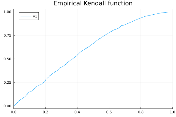

We can also visualize the ECDF of the intermediate variables Z (whose empirical CDF is K):

using StatsBase
EC = ecdf(K.z)
plot(t->EC(t); label="ECDF of Z", xlabel="t", ylabel="K_N(t)")
plot!(t->K(t); label="K(t)", color=:red, alpha=0.6)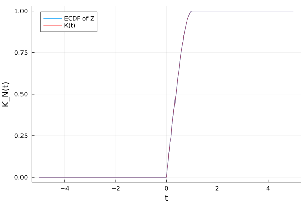

One notable detail about the Kendall function is that it does not characterize the copula in all generality. On the other hand, for an Archimedean copula with generator φ, we have:

$$K(t)=t-{\varphi }^{\prime }\{{\varphi }^{-1}(t)\}{\varphi }^{-1}(t).$$

Due to this particular relationship, the Kendall function actually characterizes the generator of the Archimedean copula. This relationship is generally expressed in terms of a λ function defined as $\lambda (t)=t-K(t),$ which, for Archimedean copulas, writes $\lambda (t)={\varphi }^{\prime }({\varphi }^{-1}(t)){\varphi }^{-1}(t)$.

Common λ functions can be easily derived by hand for standard archimedean generators. For any archimedean generator in the package, however, it is even easier to let Julia do the derivation.

Let's try to compare the empirical λ function from our dataset to a few theoretical ones. For that, we setup parameters of the relevant generators to match the kendall τ of the dataset (because we can). We include for the record the independent and completely monotonous cases.

using Copulas: ϕ⁽¹⁾, ϕ⁻¹, τ⁻¹, ClaytonGenerator, GumbelGenerator
using StatsBase: corkendall
λ(G,t) = ϕ⁽¹⁾(G,ϕ⁻¹(G,t)) * ϕ⁻¹(G,t)
plot(u -> u - K(u), xlims = (0,1), label="Empirical λ function")
κ = corkendall(x')[1,2] # empirical kendall tau
θ_cl = τ⁻¹(ClaytonGenerator,κ)
θ_gb = τ⁻¹(GumbelGenerator,κ)
plot!(u -> λ(ClaytonGenerator(θ_cl),u), label="Clayton")
plot!(u -> λ(GumbelGenerator(θ_gb),u), label="Gumbel")
plot!(u -> 0, label="Comonotony")
plot!(u -> u*log(u), label="Independence")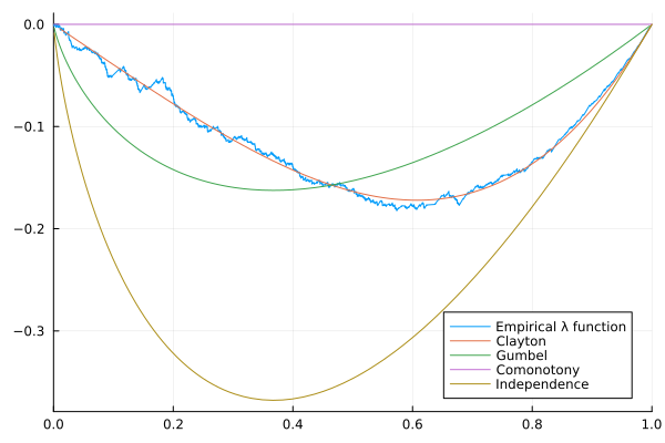

Smaller samples increase the variability of the empirical λ function. For illustration:

Xsmall = SklarDist(ClaytonCopula(2,2.7),(Normal(),Pareto()))
x2 = rand(Xsmall, 300)
K2 = KendallFunction(x2)
plot(u -> u - K(u), xlims=(0,1), label="N=1000")
plot!(u -> u - K2(u), label="N=300")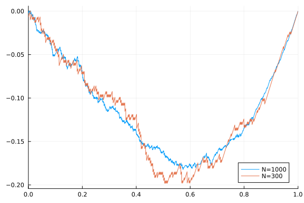

The variance of the empirical λ function is notable in this example. In particular, we note that the estimated parameter

θ_cl

2.3805798677494603

is not very far for the true $2.7$ we used to generate the dataset. A few more things could be tried before closing the analysis on a real dataset:

• Empirical validation of the Archimedean property of the data

• Non-parametric estimation of the generator from the empirical Kendall function, or through other means

• Non-Archimedean parametric models