Visualizations

Implementation details

Copulas.jl provides a dependency‑light plotting interface via Plots.jl recipes. Everything (bivariate contours/surfaces, marginal overlays, and high‑dimensional pairwise panels) is driven by keywords to the plot function.

All obj::Copula and obj::SklarDist are included in the following unified interface:

• plot(obj) gives a pairwise matrix of scatterplot of the copula/sklardist, with marginal histograms and Kendall/Spearman corelations.

• plot(obj, what) with what ∈ (:pdf, :logpdf, :cdf) – adds contour on top of the scatterplots corresponding to the pdf, logpdf or cdf function respectively.

• plot(obj, what; seriestype=:surface) – For bivariate objects only : gives 3D surfaces of the pdf, cdf or logpdf.

The following keywords can be used:

• scale=:copula / :sklar : When plotting a SklarDist, can be used to set the scale of the main scatterplots.

• show_marginals = true/false: Set to true to show histograms of the marginals (in bivariate plots only). Defaults to true for obj::SklarDist and false for obj::Copula.

• n=1500: Number of points in the scatterplots.

• bins=40: Number of bins in the histograms.

• pts_alpha=0.3 the alpha for the scatterplot.

• overlay_n=60 the grid size used for contour/surface evaluation.

• show_axes=true: set to false to hide the axes

• marg_alpha=0.6: alpha to fill the histograms.

• show_corr=true: show the Kendall/Spearman bivariate values.

All standard Plots.jl options (colors, levels, colorbar, size, themes, etc.) are available. Surfaces respect colorbar=true if set; contours suppress colorbar unless explicitly requested. Quick tips:

• Increase overlay_n for smoother contours/surfaces (cost grows ~ O(overlay_n²)). Increase n for denser scatter.

• Omit what to hide the contour/surface and view only the scatter.

• Set colorbar=true to add a colorbar (contours default to none).

• Upper triangle correlation text is centered; adjust globally with annotationfontsize if desired.

• Diagonal KDE uses a simple Gaussian kernel (Silverman bandwidth) and is always shown on the marginals.

Examples

Let us load Copulas and Plots to ativate the extension:

using Copulas
using Plots            # ensure recipes extension loads
using Distributions    # for marginals

Bivariate Copula

A bivariate Copula can be plotted as follows:

gc = GaussianCopula(2, 0.75)
p1 = plot(gc; title="Default")
p2 = plot(gc, :pdf; title=":pdf")
p3 = plot(gc, :logpdf; title=":logpdf")
p4 = plot(gc, :cdf; title=":cdf")
plot(p1,p2,p3,p4; layout=(1,4), size=(1200,260))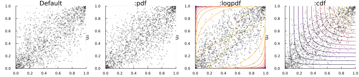

Bivariate SklarDist

For a bivaraite SklarDist, the default plot shows the scatterplot on the copula scale and add histograms of the marginals:

sd = SklarDist(GaussianCopula(2, 0.7), (Gamma(2,2), LogNormal(0.0,0.4)))
plot(sd)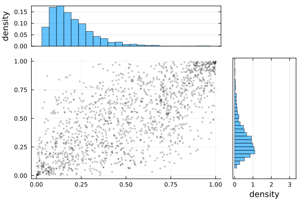

You can have the scatterplot on the marginal scales by setting scale=:sklar as well, and of course the contour by :pdf, :logpdf, :cdf still works:

# Marginal scale with marginals
plot(sd, :logpdf; scale=:sklar)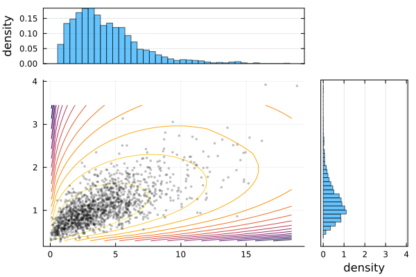

And finally you can remove the marginals by setting show_marginals=false as follows:

q1 = plot(sd;          scale=:sklar, show_marginals=false, title="Default")
q2 = plot(sd, :pdf;    scale=:sklar, show_marginals=false, title=":pdf")
q3 = plot(sd, :logpdf; scale=:sklar, show_marginals=false, title=":logpdf")
q4 = plot(sd, :cdf;    scale=:sklar, show_marginals=false, title=":cdf")
plot(q1,q2,q3, q4; layout=(1,4), size=(1200,260))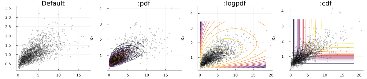

Surfaces (Copula & SklarDist)

You can obtain surface plots of bivariate copulas and sklardist as follows:

fr = FrankCopula(2, 0.8)
s1 = plot(fr, :pdf; seriestype=:surface, title=":pdf")
s2 = plot(fr, :logpdf; seriestype=:surface, title=":logpdf")
s3 = plot(fr, :cdf; seriestype=:surface, title=":cdf")
plot(s1,s2,s3; layout=(1,3), size=(1800,560))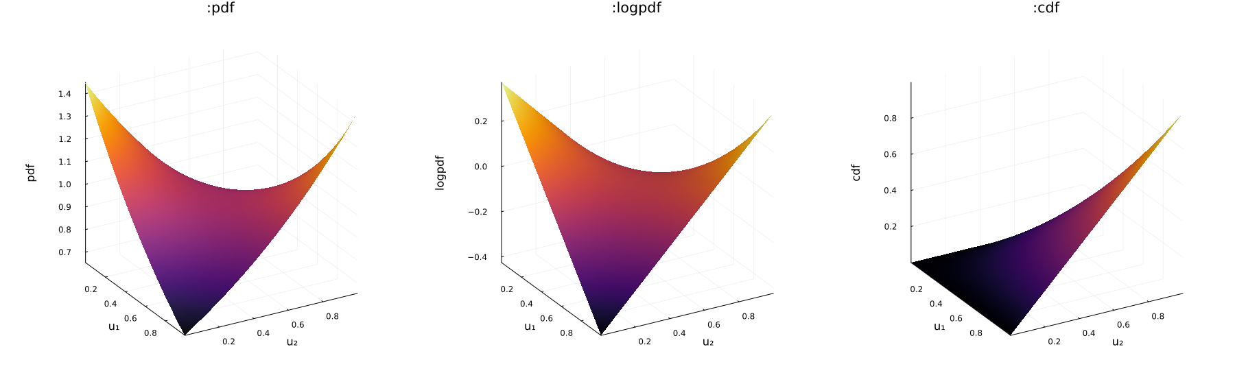

By default, the SklarDist's surfaces are on marginal scale:

sds = SklarDist(FrankCopula(2, 0.8), (Gamma(2,2), LogNormal(0.0,0.5)))
ss1 = plot(sds, :pdf; seriestype=:surface, title=":pdf")
ss2 = plot(sds, :logpdf; seriestype=:surface, title=":logpdf")
ss3 = plot(sds, :cdf; seriestype=:surface, title=":cdf")
plot(ss1,ss2,ss3; layout=(1,3), size=(1800,560))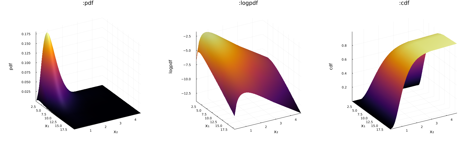

You can obtain them on copula scale by setting scale=:copula.

Pairwise Matrix – Copula

When giving a higher dimension object to the plotting function, by default you get a pairwise matrix:

c5 = FrankCopula(5, 5.0)
plot(c5)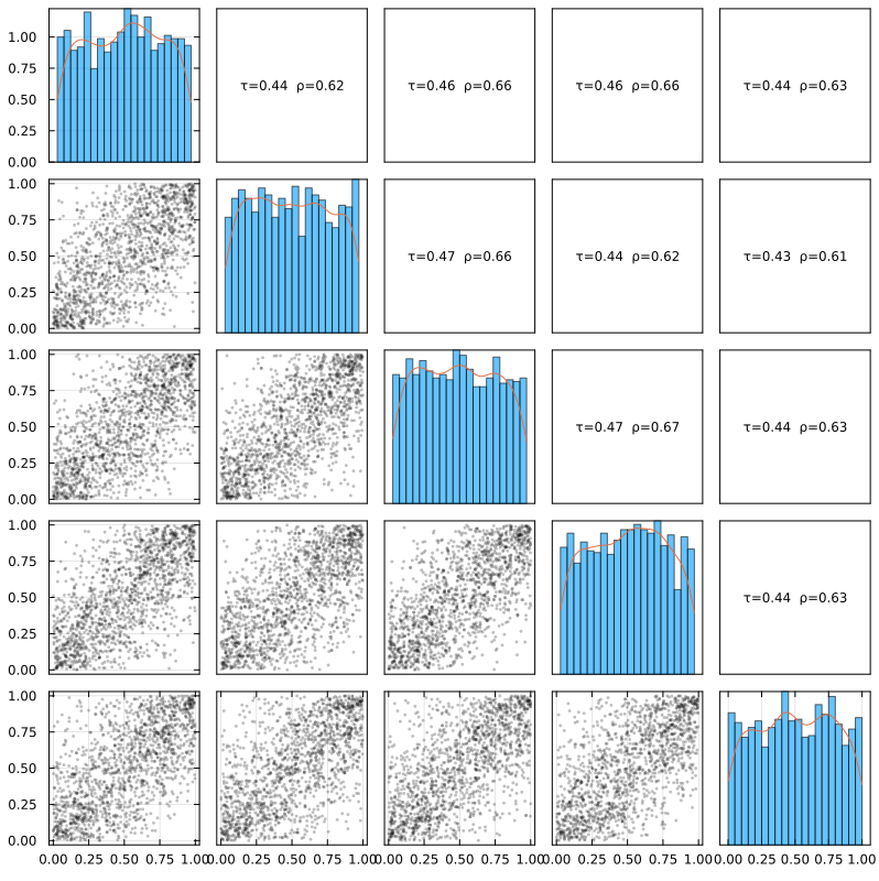

You can control of course contours by :pdf, :logpdf, :cdf, remove the correlations with show_corr=false, and a few other options (see the top of this file for their definitions)

c5 = FrankCopula(5, 12.0)
plot(c5, :pdf; show_corr=false, n=1200, overlay_n=70, pts_alpha=0.30, bins=30)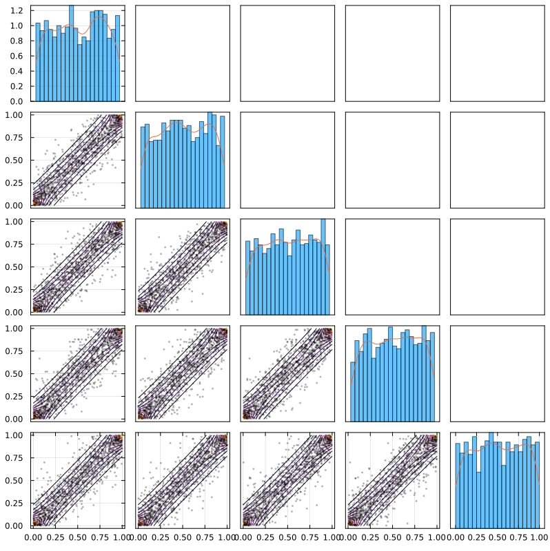

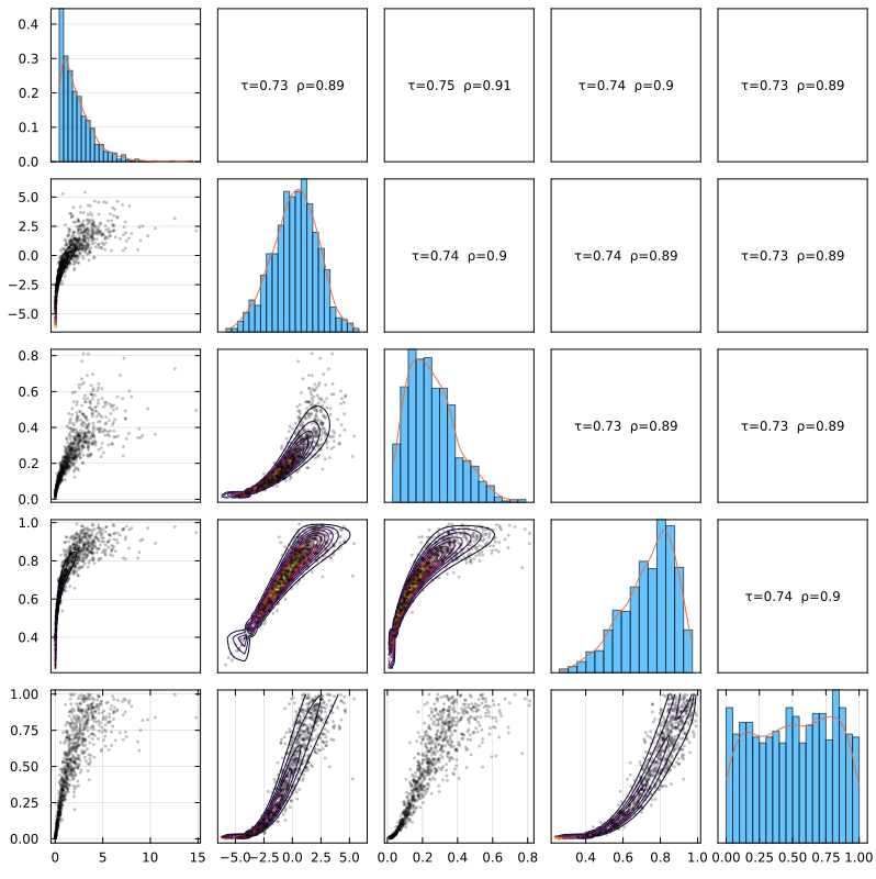
Pairwise Matrix – SklarDist

By default for a SklarDist, the scatterplots are on copula scale:

SD5 = SklarDist(ClaytonCopula(5, 6.0), (Gamma(1,2), Normal(0,2), Beta(2,6), Beta(6,2), Uniform()))
plot(SD5, :pdf; n=800, overlay_n=60, pts_alpha=0.30, bins=28)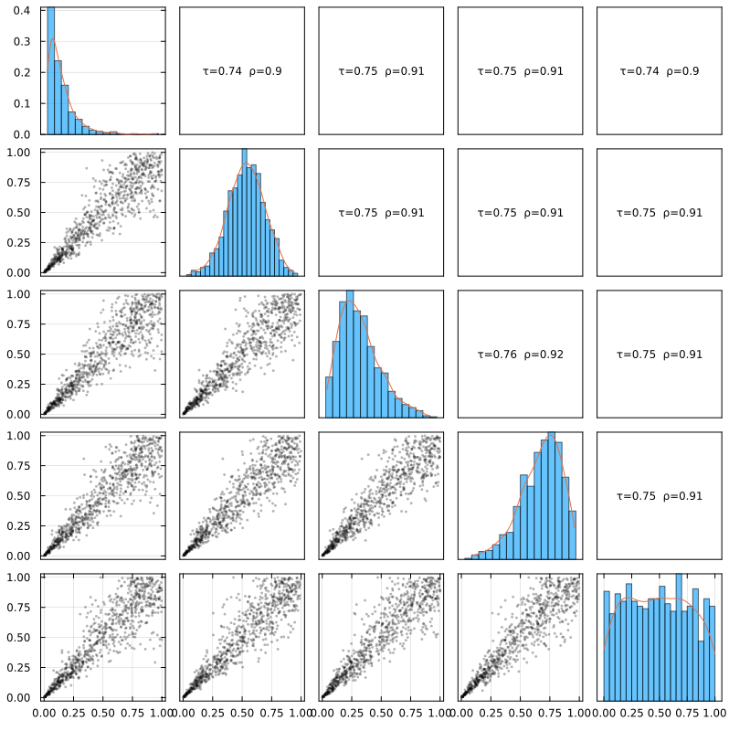

You can change the number of points and the numebr of bins of the histograms to adapt to your case:

plot(SD5; n=400, bins=12, show_corr=true)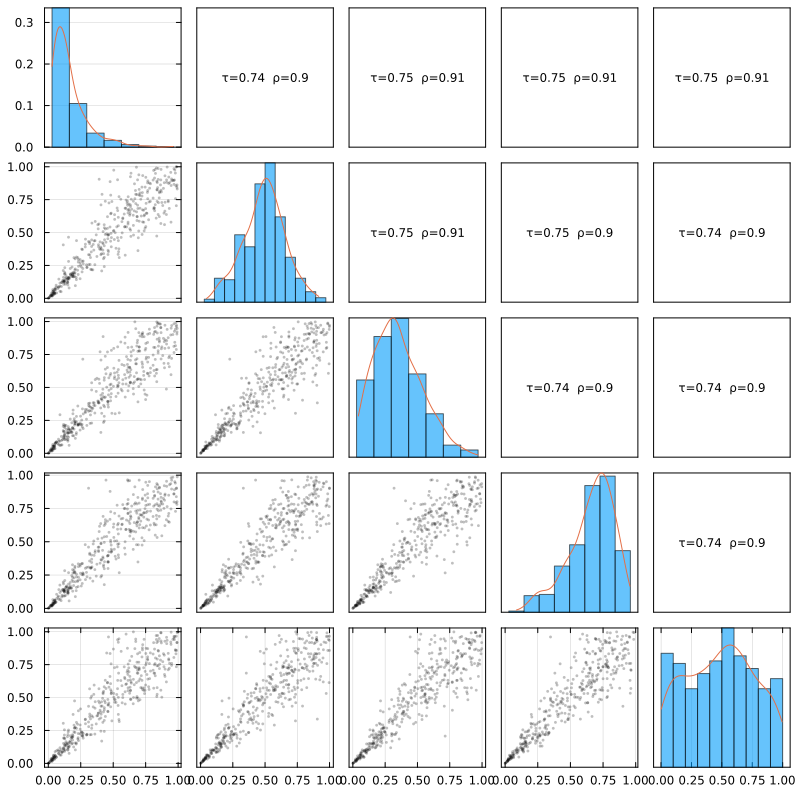

And you can also have the scatterplots on the :sklar scale

plot(SD5, :pdf; scale=:sklar, n=800, bins=28)