Bayesian inference with `Turing.jl`

Compatibility with the Distributions.jl API allows extensive interaction with the broader Julia ecosystem. One of the first examples discovered was the possibility to perform Bayesian inference of model parameters (including copulas) with Turing.jl.

Consider that we have a given model with a certain copula and certain marginals, all having parameters to be fitted. Then we can use Turing's @addlogprob! to compute the loglikelihood of our model and maximize it around the parameters alongside the chain as follows:

julia

using Copulas
using Distributions
using Random
using Turing
using StatsPlots

Random.seed!(123)
true_θ = 7
true_θ₁ = 1
true_θ₂ = 3
true_θ₃ = 2
D = SklarDist(ClaytonCopula(3,true_θ), (Exponential(true_θ₁), Pareto(true_θ₂), Exponential(true_θ₃)))
draws = rand(D, 2000)

@model function copula(X)
    # Priors
    θ  ~ TruncatedNormal(1.0, 1.0, -1/3, Inf)
    θ₁ ~ TruncatedNormal(1.0, 1.0, 0, Inf)
    θ₂ ~ TruncatedNormal(1.0, 1.0, 0, Inf)
    θ₃ ~ TruncatedNormal(1.0, 1.0, 0, Inf)

    # Build the parametric model
    C = ClaytonCopula(3,θ)
    X₁ = Exponential(θ₁)
    X₂ = Pareto(θ₂)
    X₃ = Exponential(θ₃)
    D = SklarDist(C, (X₁, X₂, X₃))

    # Compute the final loglikelyhood
    Turing.Turing.@addlogprob! loglikelihood(D, X)
end

sampler = NUTS() # MH() works too
chain = sample(copula(draws), sampler, MCMCThreads(), 100, 4)

Note that we truncated the θ parameter at -1/3 and not 0, as the ClaytonCopula can handle negative dependence structures. Only 100 steps were run for efficiency; you can increase this number as needed. The code above outputs a summary of the chain :

Summary Statistics:

parameters	true value	mean	std	mcse	ess_bulk	ess_tail	rhat	ess_per_sec
Symbol	Float64	Float64	Float64	Float64	Float64	Float64	Float64	Float64
θ	7.0	6.9319	0.1150	0.0067	291.8858	267.1353	1.0061	0.7238
θ₁	1.0	0.9954	0.0209	0.0019	116.6941	94.3070	1.0347	0.2894
θ₂	3.0	2.9839	0.0639	0.0062	108.9185	105.5284	1.0390	0.2701
θ₃	2.0	2.0055	0.0418	0.0039	114.7324	109.5396	1.0328	0.2845

Quantiles:

parameters	2.5%	25.0%	50.0%	75.0%	97.5%
Symbol	Float64	Float64	Float64	Float64	Float64
θ	6.7286	6.8438	6.9330	7.0150	7.1436
θ₁	0.9555	0.9818	0.9953	1.0093	1.0386
θ₂	2.8606	2.9426	2.9859	3.0196	3.1186
θ₃	1.9254	1.9758	2.0056	2.0336	2.0923

And then plot(chain) produces the following plot:

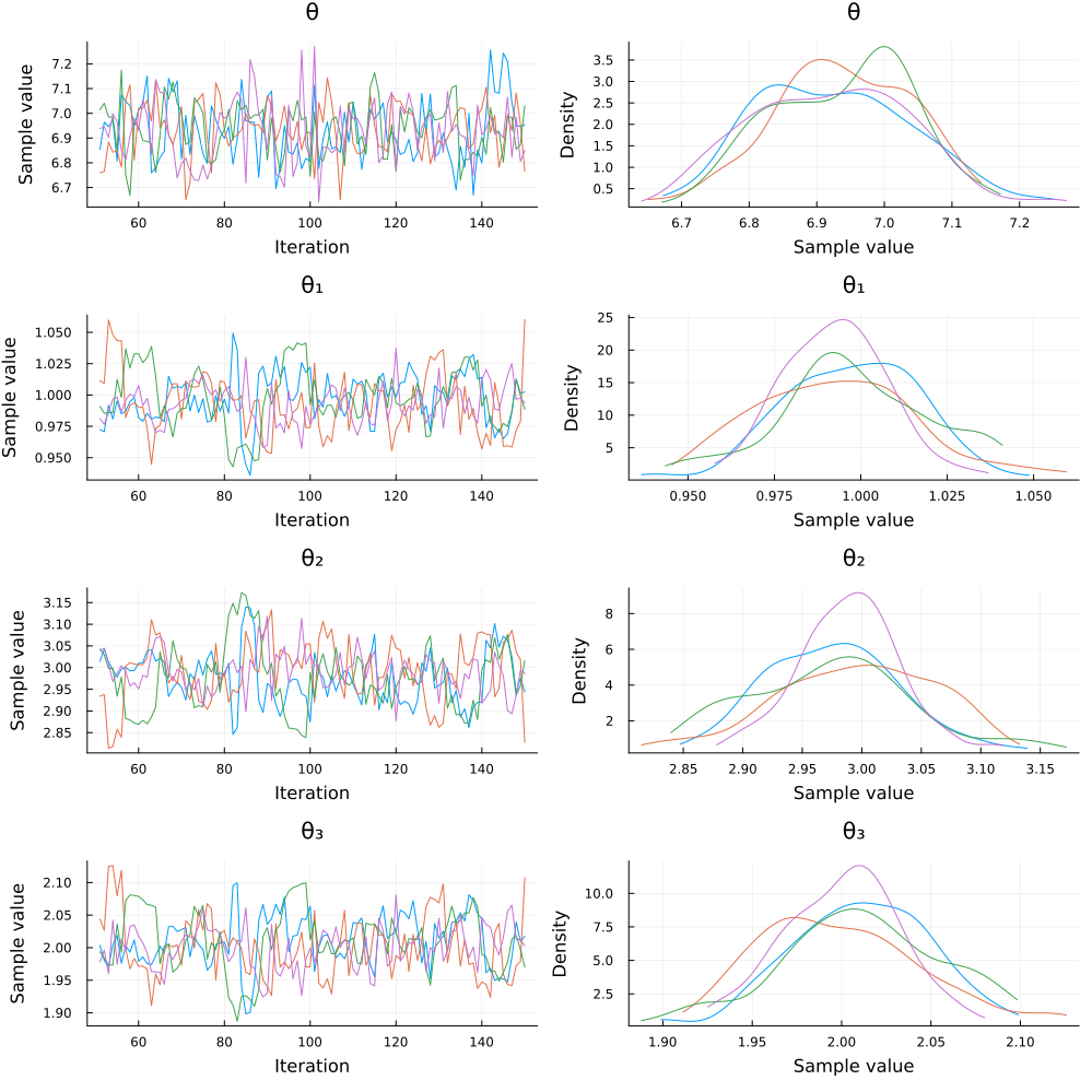
Similar approaches can be used to fit many other dependence structures in a Bayesian setting. The example above showcases parametric estimation of a sampling model, but Bayesian regression with an error structure given by a parametric copula is just as easy to implement.

This was run on the following environment:

julia

julia> versioninfo()
Julia Version 1.10.0
Commit 3120989f39 (2023-12-25 18:01 UTC)
[...]

(env) pkg> status
  [ae264745] Copulas v0.1.20
  [31c24e10] Distributions v0.25.107
  [f3b207a7] StatsPlots v0.15.6
  [fce5fe82] Turing v0.30.3
  [9a3f8284] Random

Bayesian inference with Turing.jl ​

Bayesian inference with `Turing.jl`