Conditioning and Subsetting

Conditioning

This page introduces conditional distributions under a copula model and shows how to construct them programmatically using condition. The same interface works either on the uniform scale (copula only) or on the original scale (via SklarDist).

Overview

Take a D-variate copula $C$ and consider a split of the indices $1,..,d$ into $J=1,...,p$ and $I=p+1,..,d$ wihtout loss of generality (reorder the marignals if necessary). The conditional joint distribution of the I's given the J's is given, on the uniform scale, by the function

$$H_{I\mid J}({\mathbf{u}}_I\mid {\mathbf{u}}_J):=\frac{{\partial }^{p}C({\mathbf{u}}_I,{\mathbf{u}}_J)}{\partial {\mathbf{u}}_J}/\frac{{\partial }^{p}C({\mathbf{1}}_I,{\mathbf{u}}_J)}{\partial {\mathbf{u}}_J},$$

which is a proper distribution on $[0,1{]}^{|I|}$. Each conditional marginal (uniform scale) can moreover be expressed as a “distortion” $H_{i|J}(·|u_J)$, which is the distribution function of a random variable with support $[0,1]$ (but non-uniform):

$$H_{i\mid J}(u\mid {\mathbf{u}}_J):=\frac{{\partial }^{p}C({\mathbf{u}}^{(i)}(u_I),{\mathbf{u}}_J)}{\partial {\mathbf{u}}_J}/\frac{{\partial }^{p}C(\mathbf{1},{\mathbf{u}}_J)}{\partial {\mathbf{u}}_J},$$

where ${\mathbf{u}}^{(i)}(u_I)$ has coordinate u at index i and 1 elsewhere in I.

On the original scale for a compound distribution X = SklarDist(C, (X_1,…,X_D)), conditioning on values $x_J$ is obtained by mapping to uniforms $u_J=(F_j(x_j){)}_{j\in J}$ then pushing forward each distortion through the corresponding marginal:

$$F_{X_i\mid X_J}(x\mid {\mathbf{x}}_J)=H_{i\mid J}(F_i(x)\mid {\mathbf{u}}_J).$$

The copula of the conditional vector $U_I|U_J=u_J$ is a genuine copula denoted $C_{I|J}(·|u_J)$, which is the copula of $H_{I|J}$. In our implementation, this is materialized by the a ConditionalCopula(C, J, u_J) and used internally by condition. The condition function can be used as follows:

• condition(C::Copula, js, u_js) returns the conditional distribution on the uniform scale for I = setdiff(1:D, js). If length(I) == 1, the result is a univariate distribution supported on $[0,1]$, subclass of Distortion, and otherwise it is a SklarDist(::ConditionalCopula, NTuple{d,<:Distortion}).

• condition(X::SklarDist, js, x_js) returns the conditional distribution on the original scale by pushing forward each distortion through the corresponding marginal.

• For known parametric families, there are fast paths implemented mostly as subclass to Distortions or ConditionalCopula, but this should be completely transparent to the user.

Tip: Missing fast-paths?

If you find a conditional that should admit a faster closed-form or semi-analytic path but currently falls back to the generic construction, please open an issue, we’ll happily implement it 😃

Examples

Let us visualize a given univariate distortion:

using Copulas, Distributions, Plots, StatsBase
C = ClaytonCopula(2, 1.5)
D = condition(C, 2, 0.3)  # distortion for U₁ | U₂ = 0.3
ts = range(0.0, 1.0; length=401)
plt = plot(ts, cdf.(Ref(D), ts);
          xlabel="u", ylabel="H_{1|2}(u | 0.3)",
          title="Conditional CDF on the uniform scale",
          legend=false)
plt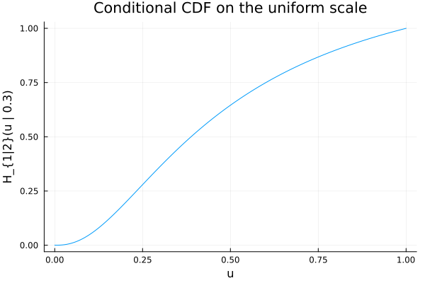

Confirm the result by overlaying the empirical cdf of a sample:

N = 2000
αs = rand(N)
us = Distributions.quantile.(Ref(D), αs)
ECDF = ecdf(us)
plot!(ts, ECDF.(ts); seriestype=:steppost, label="empirical", alpha=0.6, color=:black)
plot!(ts, cdf.(Ref(D), ts); label="analytic", color=:blue)
plt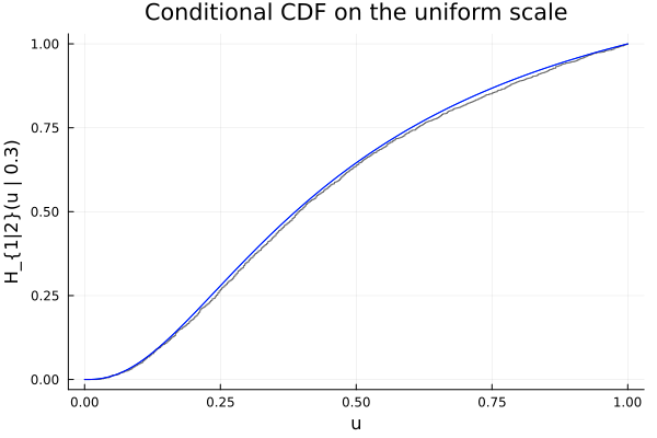

The same thing can be done on marginal scales using SklarDist:

C = ClaytonCopula(2, 1.5)
X = SklarDist(C, (Normal(), Normal()))
X1_given_X2 = condition(X, 2, 0.0) # distribution of X₁ | X₂ = 0.0
cdf(X1_given_X2, 1.0), quantile(X1_given_X2, 0.95)

(0.8472337930319087, 1.5990201973152853)

xs = rand(X1_given_X2, 2000)
Fx = ecdf(xs)
xs_grid = range(quantile(X1_given_X2, 0.001), quantile(X1_given_X2, 0.999); length=401)
plot(xs_grid, Distributions.cdf.(Ref(X1_given_X2), xs_grid);
  xlabel="x", ylabel="F_{X₁|X₂}(x|0)", title="Original-scale conditional CDF", label="analytic")
plot!(xs_grid, Fx.(xs_grid); seriestype=:steppost, label="empirical", alpha=0.6, color=:black)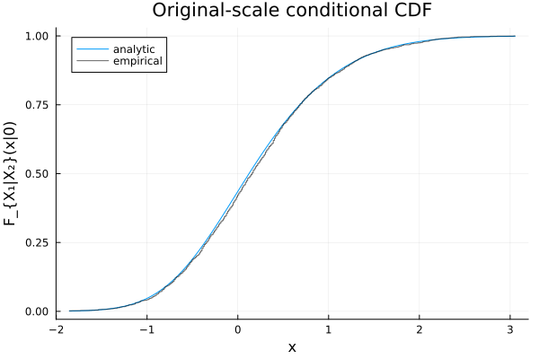

When conditioning on less than $D-1$ dimensions, we obtain a multivariate object, usually a SklarDist:

H = condition(ClaytonCopula(4, 4.2), (2, 3), (0.25, 0.8))

SklarDist{ArchimedeanCopula{2, TiltedGenerator{Copulas.ClaytonGenerator{Float64}, Float64, 2}}, Tuple{Copulas.ArchimedeanDistortion{Copulas.ClaytonGenerator{Float64}, Float64, 2}, Copulas.ArchimedeanDistortion{Copulas.ClaytonGenerator{Float64}, Float64, 2}}}(
C: ArchimedeanCopula{2, TiltedGenerator{Copulas.ClaytonGenerator{Float64}, Float64, 2}}(θ = 4.2, sJ = 80.55877526114394)
m: (Copulas.ArchimedeanDistortion{Copulas.ClaytonGenerator{Float64}, Float64, 2}(
G: Copulas.ClaytonGenerator{Float64}(4.2)
sJ: 80.55877526114394
den: 1.1276684721576129e-5
)
, Copulas.ArchimedeanDistortion{Copulas.ClaytonGenerator{Float64}, Float64, 2}(
G: Copulas.ClaytonGenerator{Float64}(4.2)
sJ: 80.55877526114394
den: 1.1276684721576129e-5
)
)
)

plot(H)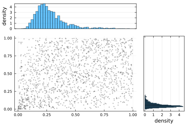

Relation to the conditional copula

The conditional copula $C_{I|J}(·|u_J)$ is the copula of the conditional distribution $H_{I|J}(·|u_J)$. In the implementation it is represented by ConditionalCopula(C, js, u_js) and is used as the copula of the conditional joint when |I| > 1. When condition returns a SklarDist (i.e., when |I| > 1), you can access this copula directly via the .C field of the returned object:

H.C # the copula

ArchimedeanCopula{2, TiltedGenerator{Copulas.ClaytonGenerator{Float64}, Float64, 2}}(θ = 4.2, sJ = 80.55877526114394)

H.m # the marginals

(Copulas.ArchimedeanDistortion{Copulas.ClaytonGenerator{Float64}, Float64, 2}(
G: Copulas.ClaytonGenerator{Float64}(4.2)
sJ: 80.55877526114394
den: 1.1276684721576129e-5
)
, Copulas.ArchimedeanDistortion{Copulas.ClaytonGenerator{Float64}, Float64, 2}(
G: Copulas.ClaytonGenerator{Float64}(4.2)
sJ: 80.55877526114394
den: 1.1276684721576129e-5
)
)

Implementation

Copulas.condition Function

    condition(C::Copula{D}, js, u_js)
    condition(X::SklarDist, js, x_js)

Construct conditional distributions with respect to a copula, either on the uniform scale (when passing a Copula) or on the original data scale (when passing a SklarDist).

Arguments

• C::Copula{D}: D-variate copula

• X::SklarDist: joint distribution with copula X.C and marginals X.m

• js: indices of conditioned coordinates (tuple, NTuple, or vector)

• u_js: values in [0,1] for U_js (when conditioning a copula)

• x_js: values on original scale for X_js (when conditioning a SklarDist)

• j, u_j, x_j: 1D convenience overloads for the common p = 1 case

Returns

• If the number of remaining coordinates d = D - length(js) is 1:

  • condition(C, js, u_js) returns a Distortion on [0,1] describing U_i | U_js = u_js.

  • condition(X, js, x_js) returns an unconditional univariate distribution for X_i | X_js = x_js, computed as the push-forward D(X.m[i]) where D = condition(C, js, u_js) and u_js = cdf.(X.m[js], x_js).

• If d > 1:

  • condition(C, js, u_js) returns the conditional joint distribution on the uniform scale as a SklarDist(ConditionalCopula, distortions).

  • condition(X, js, x_js) returns the conditional joint distribution on the original scale as a SklarDist with copula ConditionalCopula(C, js, u_js) and appropriately distorted marginals D_k(X.m[i_k]).

Notes

• For best performance, pass js and u_js as NTuple to keep p = length(js) known at compile time. The specialized method condition(::Copula{2}, j, u_j) exploits this for the common D = 2, d = 1 case.

• Specializations are provided for many copula families (Independent, Gaussian, t, Archimedean, several bivariate families). Others fall back to an automatic differentiation based construction.

• This function returns the conditional joint distribution H_{I|J}(· | u_J). The “conditional copula” is ConditionalCopula(C, js, u_js), i.e., the copula of that conditional distribution.

source

Copulas.Distortion Type

Distortion <: Distributions.ContinuousUnivariateDistribution

Abstract super-type for objects describing the (uniform-scale) conditional marginal transformation U_i | U_J = u_J of a copula.

Subtypes implement cdf/quantile on [0,1]. They are not full arbitrary distributions; they model how a uniform variable is distorted by conditioning. They can be applied as a function to a base marginal distribution to obtain the conditional marginal on the original scale: if D::Distortion and X::UnivariateDistribution, then D(X) is the distribution of X_i | U_J = u_J.

source

Copulas.DistortionFromCop Type

DistortionFromCop{TC,p,T} <: Distortion

Generic, uniform-scale conditional marginal transformation for a copula.

This is the default fallback (based on mixed partial derivatives computed via automatic differentiation) used when a faster specialized Distortion is not available for a given copula family.

Parameters

• TC: copula type

• p: length of the conditioned index set J (static)

• T: element type for the conditioned values u_J

Construction

• DistortionFromCop(C::Copula, js::NTuple{p,Int}, ujs::NTuple{p,<:Real}, i::Int) builds the distortion for the conditional marginal of index i given U_js = ujs.

Notes

• A convenience method DistortionFromCop(C, j::Int, uj::Real, i::Int) exists for the common p = 1 case.

source

Copulas.DistortedDist Type

DistortedDist{Disto,Distrib} <: Distributions.UnivariateDistribution

Push-forward of a base marginal by a Distortion.

source

Copulas.ConditionalCopula Type

ConditionalCopula{d} <: Copula{d}

Copula of the conditioned random vector U_I | U_J = u_J.

source

See also

• condition — reference documentation with all calling syntaxes

• SklarDist — compound distributions via Sklar’s theorem

• rosenblatt — sequential transforms (related but different)

Subsetting

Subsetting extracts the dependence structure among a subset of coordinates. Given a copula C of dimension d and an index tuple dims::NTuple{p,Int}, the function subsetdims returns a copula on those p dimensions that preserves the original dependence restricted to dims.

There are two entry points:

• subsetdims(C::Copula, dims) returns a Copula{p} (or Uniform() when p == 1).

• subsetdims(X::SklarDist, dims) returns a SklarDist with copula subsetdims(C, dims) and marginals (m[i] for i in dims).

Internally, we materialize subsetting with a small wrapper type SubsetCopula{p}(C, dims) which delegates cdf, pdf, and sampling to the base copula by saturating non-selected coordinates at 1. For many families we provide specialized constructors that return the natural reduced-parameter form instead of a wrapper (e.g., elliptical copulas return the appropriate submatrix, Archimedean keeps the same generator with reduced dimension, etc.). It can be used as follows:

using Copulas, Distributions
C = GaussianCopula([1.0 0.6 0.2; 0.6 1.0 0.3; 0.2 0.3 1.0])
S = subsetdims(C, (1,3))    # 2D copula on coordinates 1 and 3
length(S), typeof(S)

(2, GaussianCopula{2, Matrix{Float64}})

X = SklarDist(C, (Normal(), Normal(1,2), LogNormal()))
X13 = subsetdims(X, (1,3))  # keeps marginals (Normal(), LogNormal()) and reduces the copula
length(X13.C), length(X13.m)

(2, 2)

The resulting object depends on the copula familly, since some fast paths are given. If no specialization exists, a SubsetCopula wrapper is returned. It’s fully usable and equivalent from an API perspective; specialized forms simply yield better performance and clearer display.

Subsetting and conditioning commute in the obvious way: conditioning on coordinates J and then extracting a subset of the remaining coordinates is equivalent to subsetting the base copula first and then conditioning on the corresponding indices. In code, if S = subsetdims(C, dims), conditioning on indices js within S is implemented by mapping js to indices in the base copula and delegating to ConditionalCopula(C, ·, ·); the resulting conditional copula of S is either the base conditional copula (when all remaining coordinates are kept) or a further SubsetCopula of it.

Examples

# Archimedean example
C = ClaytonCopula(3, 2.0)
S = subsetdims(C, (1,2))        # still a ClaytonCopula with the same parameter
rand(S, 3)                      # sample 3 points
cdf(S, [0.7, 0.9])

0.6629375642933931

# Survival example with flips remapped
base = GaussianCopula([1.0 0.7 0.2; 0.7 1.0 0.1; 0.2 0.1 1.0])
S = SurvivalCopula(base, (2,))
S13 = subsetdims(S, (1,3))      # flip on 2 drops; no flips remain
typeof(S13), S13 isa SurvivalCopula

(GaussianCopula{2, Matrix{Float64}}, false)

Implementation

Copulas.subsetdims Function

subsetdims(C::Copula, dims::NTuple{p, Int})
subsetdims(D::SklarDist, dims)

Return a new copula or Sklar distribution corresponding to the subset of dimensions specified by dims.

Arguments

• C::Copula: The original copula object.

• D::SklarDist: The original Sklar distribution.

• dims::NTuple{p, Int}: Tuple of indices representing the dimensions to keep.

Returns

• A SubsetCopula or a new SklarDist object corresponding to the selected dimensions. If p == 1, returns a Uniform distribution or the corresponding marginal.

Details

This function extracts the dependence structure among the specified dimensions from the original copula or Sklar distribution. Specialized methods exist for some copula types to ensure efficiency and correctness.

source

Copulas.SubsetCopula Type

SubsetCopula{d,CT}

Fields:

• C::CT - The copula

• dims::Tuple{Int} - a Tuple representing which dimensions are used.

Constructor

SubsetCopula(C::Copula,dims)

This class allows to construct a random vector corresponding to a few dimensions of the starting copula. If $(X_1,...,X_n)$ is the random vector corresponding to the copula C, this returns the copula of ( $X_i$ for i in dims). The dependence structure is preserved. There are specialized methods for some copulas.

source

Rosenblatt transformations

Definition and usefulness

Definition: Rosenblatt transformation

The Rosenblatt transformation considers a random vector $X$ distributed according to a certain multivariate cumulative distribution function $F_X(x)$, and maps it back to a uniform distribution on the unit hypercube.

More formally, consider the map $R_X(x)$ defined as follows:

$$R_X(x_1,...,x_d)=(r_1=F_{X_1}(x_1),r_2=F_{X_2|X_1}(x_2|x_1),...,r_d=F_{X_d|X_1,...,X_{d-1}}(x_d|x_1,...,x_{d-1}))$$

References:

• [13] Rosenblatt, M. (1952). Remarks on a multivariate transformation. Annals of Mathematical Statistics, 23(3), 470-472.

• [4] Joe, H. (2014). Dependence Modeling with Copulas. CRC Press. (Section 2.10)

• [14] McNeil, A. J., & Nešlehová, J. (2009). Multivariate Archimedean copulas, d-monotone functions and ℓ 1-norm symmetric distributions.

In certain circumstances, in particular for Archimedean copulas, this map simplifies to tractable expressions. It has a few nice properties:

• $R_X(X)\sim \mathtt{\text{Uniform(Unit Hypercube)}}$

• $R_X$ is a bijection.

These two properties are leveraged in some cases to construct the inverse Rosenblatt transformations, which map random noise to proper samples from the copula. In some cases, this is the best sampling algorithm available.

Implementation

As soon as the random vector $X$ is represented by an object X that subtypes SklarDist or Copula, you have access to the rosenblatt(X, x) and inverse_rosenblatt(X, x) operators, which both have a straightforward interpretation from their names.

Copulas.rosenblatt Function

rosenblatt(C::Copula, u)

Computes the rosenblatt transform associated to the copula C on the vector u. Formally, assuming that U ∼ C, the result should be uniformely distributed on the unit hypercube. The importance of this transofrmation comes from its bijectivity: inverse_rosenblatt(C, rand(d)) is equivalent to rand(C). The interface proposes faster versions for matrix inputs u.

Generic Rosenblatt transform using conditional distortions: S₁ = U₁, S_k = H_{k|1:(k-1)}(U_k | U₁:U_{k-1}). Specialized families may provide faster overrides.

• [13] Rosenblatt, M. (1952). Remarks on a multivariate transformation. Annals of Mathematical Statistics, 23(3), 470-472.

• [4] Joe, H. (2014). Dependence Modeling with Copulas. CRC Press. (Section 2.10)

• [14] McNeil, A. J., & Nešlehová, J. (2009). Multivariate Archimedean copulas, d-monotone functions and ℓ 1-norm symmetric distributions.

source

Copulas.inverse_rosenblatt Function

inverse_rosenblatt(C::Copula, u)

Computes the inverse rosenblatt transform associated to the copula C on the vector u. Formally, assuming that U ∼ Π, the independence copula, the result should be distributed as C. Also look at rosenblatt(C, u) for the inverse transformation. The interface proposes faster versions for matrix inputs u.

Generic inverse Rosenblatt using conditional distortions: U₁ = S₁, U_k = H_{k|1:(k-1)}^{-1}(S_k | U₁:U_{k-1}). Specialized families may provide faster overrides.

References:

• [13] Rosenblatt, M. (1952). Remarks on a multivariate transformation. Annals of Mathematical Statistics, 23(3), 470-472.

• [4] Joe, H. (2014). Dependence Modeling with Copulas. CRC Press. (Section 2.10)

• [14] McNeil, A. J., & Nešlehová, J. (2009). Multivariate Archimedean copulas, d-monotone functions and ℓ 1-norm symmetric distributions.

source

Once again, since the rosenblatt transform leverages the conditioning mechanisme, some fast-paths might be missing in the implementation.

Sanity check plot

You can validate that the Rosenblatt transform maps samples to independent uniforms by checking the marginal ECDFs against the 45° line.

using Copulas, Plots, StatsBase
# pick a nontrivial copula
C = ClaytonCopula(3, 1.5)

# draw samples and apply Rosenblatt transform coordinate-wise
U = rand(C, 3000)                 # size (3, N)
S = reduce(hcat, (rosenblatt(C, U[:, i]) for i in 1:size(U, 2)))  # size (3, N)

ts = range(0.0, 1.0; length=401)
layout = @layout [a b c]
plt = plot(layout=layout, size=(900, 280), legend=false)
for k in 1:3
  Ek = ecdf(S[k, :])
  plot!(plt[k], ts, Ek.(ts); seriestype=:steppost, color=:black,
      title="ECDF of $(k)", xlabel="u", ylabel="ECDF")
  plot!(plt[k], ts, ts; color=:blue, alpha=0.7)
end
plt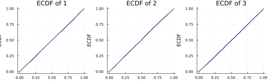

References

1. H. Joe. Dependence Modeling with Copulas (CRC press, 2014).

2. M. Rosenblatt. Remarks on a multivariate transformation. Annals of Mathematical Statistics 23, 470–472 (1952).

3. A. J. McNeil and J. Nešlehová. Multivariate Archimedean Copulas, d -Monotone Functions and L1 -Norm Symmetric Distributions. The Annals of Statistics 37, 3059–3097 (2009).