Dependence measures

The copula of a random vector fully encodes its dependence structure. However, copulas are infinite-dimensional objects and interpreting their properties can be difficult as the dimension increases. Therefore, the literature has introduced quantifications of the dependence structure that may be used as univariate (imperfect but useful) summaries of certain copula properties. We implement the most well-known ones in this package.

Main dependence metrics τ, ρ, β and γ

Definition: Kendall' τ

For a copula $C$ with a density $c$, regardless of its dimension $d$, Kendall's τ is defined as:

$$\tau =\frac{2^d}{2^{d-1}-1}\int C(\mathit{u})c(\mathit{u})d\mathit{u}-\frac{1}{2^{d-1}-1}$$

Definition: Spearman's ρ

For a copula $C$ with a density $c$, regardless of its dimension $d$, Spearman's ρ is defined as:

$$\rho =\frac{2^d\ast (d+1)}{2^d-d-1}\int C(\mathit{u})d\mathit{u}-\frac{d+1}{2^d-(d+1)}.$$

Definition: Definition (Blomqvist's β):

For a copula $C$ with a density $c$, regardless of its dimension $d$, Blomqvist's β is defined as:

$$\beta =\frac{2^{d-1}}{2^{d-1}-1}(C(\frac{\mathbf{1}}{\mathbf{2}})+\overline{C}(\frac{\mathbf{1}}{\mathbf{2}}))-\frac{1}{2^{d-1}-1}.$$

where $\overline{C}$ is the survival copula associated with $C$.

Definition: Definition (Gini's γ):

For a copula $C$ with a density $c$, regardless of its dimension $d$, the multivariate Gini’s gamma is defined as [15]:

$$\gamma =\frac{1}{b(d)-a(d)}[{\int }_{[0,1{]}^d}\{A(\mathit{u})+\overline{A}(\mathit{u})\}dC(\mathit{u})-a(d)],$$

with

$$A(u)=\frac{1}{2}(min(u)+max(\sum _{i=1}^d{u}_i-d+1,0)),\overline{A}(u)=\frac{1}{2}(1-max(u)+max(1-\sum _{i=1}^d{u}_i,0)),$$

while $a_d,b_d$ are normalizing constants depending only on the dimension $d$.

These dependence measures are very common when $d=2$, and a bit less when $d>2$. We sometimes refer to the Kendall's matrix or the Spearman's matrix for the collection of bivariate coefficients associated with a multivariate copula. We thus provide two different interfaces:

• Copulas.τ(C::Copula), Copulas.ρ(C::Copula), Copulas.β(C::Copula), Copulas.γ(C::Copula) provide the upper formulas, yielding a scalar whatever the dimension of the copula.

• StatsBase.corkendall(data), StatsBase.corspearman(data), Copulas.corblomqvist(data), Copulas.corgini(data) provide matrices of pairwise dependence metrics.

Thus, for a given copula C, the theoretical dependence measures can be obtained by τ(C), ρ(C), β(C), γ(C) (for the multivariate versions) and corkendall(C), corspearman(C), corblomqvist(C), and corgini(C) (for the matrix versions). Similarly, empirical versions of these metrics can be obtained from a matrix of observations data of size (d,n) by Copulas.τ(data), Copulas.ρ(data), Copulas.β(data), Copulas.γ(data), StatsBase.corkendall(data), StatsBase.corspearman(data), Copulas.corblomqvist(data) and Copulas.corgini(data).

Tip: Ranges of τ, ρ, β and γ.

Kendall's $\tau$, Spearman's $\rho$, Blomqvist's $\beta$ and Gini's $\gamma$ all belong to $[-1,1]$. They are equal to :

• 0 if and only if the copula is a IndependentCopula.

• -1 is and only if the copula is a WCopula.

• 1 if and only if the copula is a MCopula.

They do not depend on the marginals. This is why we say that they measure the 'strength' of the dependency.

Todo: Work in progress

The package implements generic version of the dependence metrics, but some families have faster versions (closed form formulas or better integration paths). However, all the potential fast-paths are not implemented yet. If you feel a specific method for a certain copula is missing, do not hesitate to open an issue !

Moreover, many copula estimators are based on the relationship between parameters and these coefficients (see e.g., [16–18]), but once again our implementation is not complete yet.

Here is for example the relationship between the Kendall $\tau$ and the parameter of a Clayton copula:

using Copulas, Plots, Distributions
θs = -1:0.1:5
τs = [Copulas.τ(ClaytonCopula(2, θ)) for θ in θs]
plot(θs, τs; xlabel="θ", ylabel="τ", title="θ -> τ for bivariate Clayton", legend=false)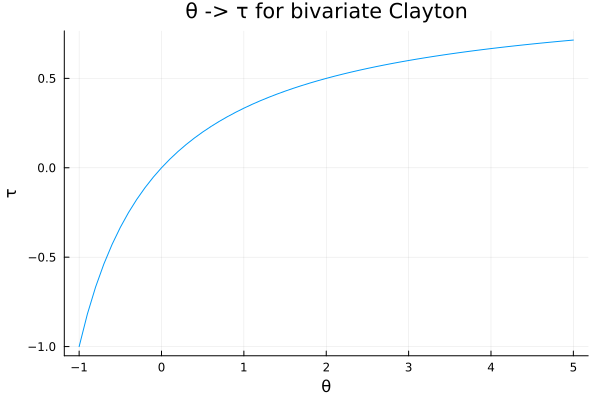

Remark the clear and easy to exploit bijection.

Info: Efficiency note

In practice, Gini’s γ is the most efficient dependence measure in our implementation (microseconds, no allocations). Kendall’s τ is the most computationally expensive ((O(n^2))), while Spearman’s ρ and Blomqvist’s β are intermediate. For pairwise matrices, corgini is faster than both corblomqvist and the classical corspearman/corkendall.

Tail dependency

Many people are interested in the tail behavior of their dependence structures. Tail coefficients summarize this tail behavior.

Definition: Tail dependency

For a copula $C$, we define the upper tail statisticss (when they exist):

$$\begin{array}{rl}{\lambda }_U(u)& =\frac{1-2u-C(u,..,u)}{1-u}\\ {\lambda }_U& =\underset{u\to 1_{-}}{lim}{\lambda }_U(u)\in [0,1]\\ {\chi }_U(u)& =\frac{2\ln (1-u)}{\ln (1-2u+C(u,...,u))}-1\\ {\chi }_U& =\underset{u\to 1_{-}}{lim}{\chi }_U(u)\in [-1,1]\end{array}$$

Simetric tools can be constructed for the lower tail:

$$\begin{array}{rl}{\lambda }_L(u)& =\frac{C(u,..,u)}{u}\\ {\lambda }_L& =\underset{u\to 0_{+}}{lim}{\lambda }_L(u)\in [0,1]\\ {\chi }_L(u)& =\frac{2\ln (u)}{\ln (C(u,...,u))}-1\\ {\chi }_L& =\underset{u\to 0_{+}}{lim}\chi (u)\in [-1,1]\end{array}$$

When ${\lambda }_U>0$ (resp ${\lambda }_L>0$), we say that there is strong upper (resp lower) tail dependency, and ${\chi }_U=1$ (resp ${\chi }_L=1$). When ${\lambda }_U>0$ (resp ${\lambda }_L>0$), if furthermore ${\chi }_U\ne 0$ (resp ${\chi }_L\ne 0$), we say that there is weak upper tail dependency. Otherwise we ay there is no tail dependency. Thus, the graph of ${\lambda }_L(u),{\chi }_L(u)$ over $[0,\frac{1}{2}]$, and the graph of ${\lambda }_U(u),{\chi }_U(u)$ over $[\frac{1}{2},1]$ are usefull tools to diagnose the potential limits.

using Copulas, Distributions, Plots
λᵤ(C::Copulas.Copula{d}, u) where d = (1 - 2u - cdf(C, fill(u,d)))/(1-u)
χᵤ(C::Copulas.Copula{d}, u) where d = 2 * log1p(- u) / log1p(- 2u + cdf(C, fill(u,d))) - 1

C = GumbelCopula(2, 2.5)
plot(0.9:0.001:0.999, Base.Fix1(λᵤ, C); xlabel="u", label="λᵤ(u)", title="Graph of λᵤ(u) and χᵤ(u)  for Gumbel Copula")
plot!(0.9:0.001:0.999, Base.Fix1(χᵤ, C); label="χᵤ(u)")

C = ClaytonCopula(2, 2.5)
plot(0.9:0.001:0.999, Base.Fix1(λᵤ, C); xlabel="u", label="λᵤ(u)", title="Graph of λᵤ(u) and χᵤ(u) for Clayton Copula")
plot!(0.9:0.001:0.999, Base.Fix1(χᵤ, C); label="χᵤ(u)")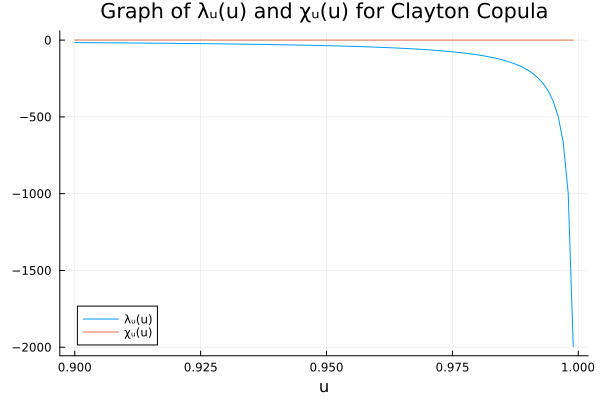

All these coefficients quantify the behavior of the dependence structure, generally or in the extremes, and are therefore widely used in the literature either as verification tools to assess the quality of fits, or even as parameters. Many parametric copula families have simple surjections, injections, or even bijections between these coefficients and their parametrization, allowing matching procedures of estimation (similar to moment matching algorithms for fitting standard random variables).

The package provides both theoretical limits (for a given copula object) and empirical estimators (from data matrices). In addition, pairwise tail-dependence matrices can be computed for multivariate samples.

• Theoretical λ: λₗ(C::Copula) and λᵤ(C::Copula) Shortcuts: λₗ(C), λᵤ(C)

• Empirical λ: λₗ(U::AbstractMatrix; p=1/√m) and λᵤ(U::AbstractMatrix; p=1/√m)

• Pairwise λ-matrix: coruppertail(data; method=:SchmidtStadtmueller, p=1/√m) and corlowertail(data; method=:SchmidtStadtmueller, p=1/√m)

These follow the approach of Schmidt & Stadtmüller (see [19]).

Todo: Work in progress

The formalization of an interface for obtaining the tail dependence coefficients of copulas is still a work in progress in the package. Do not hesitate to reach us on GitHub if you want to discuss it!

Copula entropy

Definition: Definition (Copula entropy):

For a copula $C$ with density $c$, the copula entropy:

$$\iota (C)=-{\int }_{[0,1{]}^d}c(u)\log c(u),du.$$

Ma & Sun (2011) proved that the mutual information of a random vector equals the negative copula entropy:

$$I(X_1,\dots ,X_d)=-\iota (C).$$

See [20].

Basic properties if the copula entropy:

$$\iota (C)\le 0$$

with equality $\iota (C)=0$ if and only if $C$ is the IndependentCopula (because $c\equiv 1$).

• For singular copulas (without density), $H(C)=-\mathrm{\infty }$.

• Since $I=-\iota$, the larger the $I$ $\Rightarrow$, the greater the dependence (linear, nonlinear, tailing, etc.).

Tip: the iota symbol

Remark that the iota symbol can be obtain by typing "\iota<tab>".

Our implementation proposes two options:

• Parametric (Monte Carlo): ι(C::Copula; nmc=100_000) Returns H

• Non-parametric (kNN): ι(U::AbstractMatrix; k=5, p=Inf): uses a Kozachenko–Leonenko estimator ([21]) on pseudo-observations $U\in (0,1{)}^d$. Typical parameters: $k\in [5,15]$; norm $p\in \{1,2,\mathrm{\infty }\}$.

• Pairwise version: corentropy(data; k=5, p=Inf): Matrices of $H$ for all pairs; signed=true multiplies $r$ by $\mathrm{sign}(\tau )$.

Tip: Efficiency

While $\tau$, $\rho$, $\beta$ or $\gamma$ can be computed in microseconds, entropy-based measures are much slower due to simulation or kNN search. Benchmarks confirm this: γ is fastest, whereas entropy and corentropy are orders of magnitude slower. They are therefore recommended mainly for validation, model selection, or feature screening, not routine use.

References

1. J. Behboodian, A. Dolati and M. Úbeda-Flores. A multivariate version of Gini's rank association coefficient. Statistical Papers 48, 295–304 (2007).

2. C. Genest, J. Nešlehová and N. Ben Ghorbal. Estimators Based on Kendall's Tau in Multivariate Copula Models. Australian & New Zealand Journal of Statistics 53, 157–177 (2011).

3. G. A. Fredricks and R. B. Nelsen. On the Relationship between Spearman's Rho and Kendall's Tau for Pairs of Continuous Random Variables. Journal of Statistical Planning and Inference 137, 2143–2150 (2007).

4. A. Derumigny and J.-D. Fermanian. À propos des tests de l'hypothèse simplificatrice pour les copules conditionnelles. JDS2017, 6 (2017).

5. R. Schmidt and U. Stadtmüller. Non-parametric estimation of tail dependence. Scandinavian journal of statistics 33, 307–335 (2006).

6. J. Ma and Z. Sun. Mutual information is copula entropy. Tsinghua Science and Technology 16, 51–54 (2011).

7. L. Kozachenko. Sample estimate of the entropy of a random vector. Probl. Pered. Inform. 23, 9 (1987).