Archimedean family

Archimedean copulas are an important parametric class of copulas. To define Archimedean copulas, we must consider their generators, which are unrelated to spherical generators and must be $d$-monotone functions.

Generators and d-monotony

Archimedean generators can be defined as follows:

Definition: Archimedean generator

A $d$-Archimedean generator is a $d$-monotone function

$$\varphi :{\mathbb{R}}_{+}\to [0,1]$$

such that $\varphi (0)=1$ and $\varphi (+\mathrm{\infty })=0$.

where the notion of $d$-monotone function is defined (see e.g. [14]) as follows:

Definition: d-monotony

A function $\varphi$ is $d$-monotone if it has $d-2$ derivatives which satisfy

$$(-1{)}^k{\varphi }^{(k)}\ge 0$$

for all $k\in \{1,...,d-2\}$, and if $(-1{)}^{d-2}{\varphi }^{(d-2)}$ is a non-increasing and convex function.

A function that is $d$-monotone for all $d$ is called completely monotone.

In this package, there is an abstract class Generator that contains those generators.

Tip: Available Archimedean generators

The package covers every archimedean generators that exists through a generic implementation of the Williamson d-transform, see the next section.

On the other hand, many parametric Archimedean generators are specifically implemented, see this list of implemented archimedean generator to get an overview of which ones are availiable.

Info: Empirical generator estimator

From data, you can estimate a $d$-Archimedean generator nonparametrically via the empirical Kendall distribution. The estimator is available as EmpiricalGenerator, see the empirical manual page for the method and usage.

If you do not find the generator you need, you may define it yourself by subtyping Generator. The API requires only two methods:

• The φ(G::MyGenerator, t) function returns the value of the Archimedean generator itself.

• The max_monotony(G::MyGenerator) returns its maximum monotony, i.e., the greatest integer $d$ for which the generator is $d$-monotone.

Thus, a new generator implementation may simply look like:

struct MyGenerator{T} <: Generator
    θ::T
end
ϕ(G::MyGenerator,t) = exp(-G.θ * t) # can you recognise this one ?
max_monotony(G::MyGenerator) = Inf

Tip: Win-Win strategy

These two functions are enough to sample the corresponding Archimedean copula (see the Inverse Williamson $d$-transforms section of the documentation). However, if you know more about your generator, implementing a few additional methods can greatly speed up the algorithms. More details on these methods are in the Generator docstring.

For example, Here is a graph of a few Clayton Generators:

using Copulas: ϕ,ClaytonGenerator,IndependentGenerator
using Plots
plot( x -> ϕ(ClaytonGenerator(-0.5),x), xlims=(0,5), label="ClaytonGenerator(-0.5)")
plot!(x -> exp(-x), label="IndependentGenerator()")
plot!(x -> ϕ(ClaytonGenerator(0.5),x), label="ClaytonGenerator(0.5)")
plot!(x -> ϕ(ClaytonGenerator(1),x), label="ClaytonGenerator(1)")
plot!(x -> ϕ(ClaytonGenerator(5),x), label="ClaytonGenerator(5)")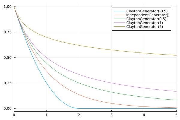

And the corresponding inverse functions:

using Copulas: ϕ⁻¹,ClaytonGenerator,IndependentGenerator
using Plots
plot( x -> ϕ⁻¹(ClaytonGenerator(-0.5),x), xlims=(0,1), ylims=(0,5), label="ClaytonGenerator(-0.5)")
plot!(x -> -log(x), label="IndependentGenerator()")
plot!(x -> ϕ⁻¹(ClaytonGenerator(0.5),x), label="ClaytonGenerator(0.5)")
plot!(x -> ϕ⁻¹(ClaytonGenerator(1),x), label="ClaytonGenerator(1)")
plot!(x -> ϕ⁻¹(ClaytonGenerator(5),x), label="ClaytonGenerator(5)")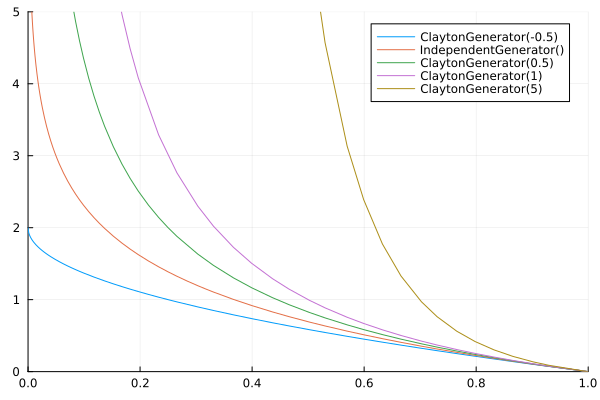

Copulas.Generator Type

Generator

Abstract type. Implements the API for archimedean generators.

An Archimedean generator is simply a function $\varphi :{\mathbb{R}}_{+}\to [0,1]$ such that $\varphi (0)=1$ and $\varphi (+\mathrm{\infty })=0$.

To generate an archimedean copula in dimension $d$, the function also needs to be $d$-monotone, that is :

• $\varphi$ is $d-2$ times derivable.

• $(-1{)}^k{\varphi }^{(k)}\ge 0\mathrm{\forall }k\in \{1,..,d-2\},$ and if $(-1{)}^{d-2}{\varphi }^{(d-2)}$ is a non-increasing and convex function.

The access to the function $\varphi$ itself is done through the interface:

ϕ(G::Generator, t)

We do not check algorithmically that the proposed generators are d-monotonous. Instead, it is up to the person implementing the generator to tell the interface how big can $d$ be through the function

max_monotony(G::MyGenerator) = # some integer, the maximum d so that the generator is d-monotonous.

More methods can be implemented for performance, althouhg there are implement defaults in the package :

• ϕ⁻¹( G::Generator, x) gives the inverse function of the generator.

• ϕ⁽¹⁾(G::Generator, t) gives the first derivative of the generator

• ϕ⁽ᵏ⁾(G::Generator, k::Int, t) gives the kth derivative of the generator

• ϕ⁻¹⁽¹⁾(G::Generator, t) gives the first derivative of the inverse generator.

• 𝒲₋₁(G::Generator, d::Int) gives the Wiliamson d-transform of the generator as a univaraite positive dsitribution.

References:

• [14] McNeil, A. J., & Nešlehová, J. (2009). Multivariate Archimedean copulas, d-monotone functions and ℓ 1-norm symmetric distributions.

source

Note that the rate at which these functions approach 0 (and their inverse approaches infinity on the left boundary) can vary significantly between generators. The difference between each is easier to see on the inverse plot.

Williamson d-transform

An easy way to construct new $d$-monotonous generators is the use of the Williamson $d$-transform.

Definition: Williamson d-transformation

For a univariate non-negative random variable $X$, with cumulative distribution function $F$ and integer $d\ge 2$, the Williamson-d-transform of $X$ is the real function supported on $[0,\mathrm{\infty }[$ given by:

$$\varphi (t)={\mathcal{W}}_d(X)(t)$$$$={\int }_t^{\mathrm{\infty }}{(1-\frac{t}{x})}^{d-1}dF(x)$$$$=\mathbb{E}((1-\frac{t}{X}{)}_{+}^{d-1}){\mathbb{1}}_{t>0}+(1-F(0)){\mathbb{1}}_{t<0}$$

In this package, we implemented it through the WilliamsonGenerator class. It can be used as follows:

WilliamsonGenerator(X::UnivariateRandomVariable, d).

This function computes the Williamson d-transform of the provided random variable $X$. See [14, 28] for the literature.

Info: `max_monotony` of Williamson generators

The $d$-transform of a positive random variable is $d$-monotone but not $k$-monotone for any $k>d$. Its max monotony is therefore $d$. This has a few implications, one of the biggest is that the $d$-variate Archimedean copula that corresponds has no density.

More generally, if you want your Archimedean copula to have a density, you must use a generator that is more-monotone than the dimension of your model.

Copulas.WilliamsonGenerator Type

WilliamsonGenerator{TX, d} (alias 𝒲{TX, d})

Fields:

• X::TX – a random variable that represents its Williamson d-transform

The type parameter d::Int is the dimension of the transformation.

Constructor

WilliamsonGenerator(X::Distributions.UnivariateDistribution, d)
𝒲(X::Distributions.UnivariateDistribution,d)
WilliamsonGenerator(atoms::AbstractVector, weights::AbstractVector, d)
𝒲(atoms::AbstractVector, weights::AbstractVector, d)

The WilliamsonGenerator (alias 𝒲) allows to construct a d-monotonous archimedean generator from a positive random variable X::Distributions.UnivariateDistribution. The transformation, which is called the inverse Williamson transformation, is implemented fully generically in the package.

For a univariate non-negative random variable $X$, with cumulative distribution function $F$ and an integer $d\ge 2$, the Williamson-d-transform of $X$ is the real function supported on $[0,\mathrm{\infty }[$ given by:

$$\varphi (t)={𝒲}_d(X)(t)={\int }_t^{\mathrm{\infty }}{(1-\frac{t}{x})}^{d-1}dF(x)=\mathbb{E}((1-\frac{t}{X}{)}_{+}^{d-1}){\mathbb{1}}_{t>0}+(1-F(0)){\mathbb{1}}_{t<0}$$

This function has several properties:

• We have that $\varphi (0)=1$ and $\varphi (Inf)=0$

• $\varphi$ is $d-2$ times derivable, and the signs of its derivatives alternates : $\mathrm{\forall }k\in 0,...,d-2,(-1{)}^k{\varphi }^{(k)}\ge 0$.

• ${\varphi }^{(d-2)}$ is convex.

These properties makes this function what is called a d-monotone archimedean generator, able to generate archimedean copulas in dimensions up to $d$. Our implementation provides this through the Generator interface: the function $\varphi$ can be accessed by

G = WilliamsonGenerator(X, d)
ϕ(G,t)

Note that you'll always have:

max_monotony(WilliamsonGenerator(X,d)) === d

Special case (finite-support discrete X)

• If X isa Distributions.DiscreteUnivariateDistribution and support(X) is finite, or if you pass directly atoms and weights to the constructor, the produced generator is piecewise-polynomial ϕ(t) = ∑_j w_j · (1 − t/r_j)_+^(d−1) matching the Williamson transform of a discrete radial law. It has specialized methods.

• For infinite-support discrete distributions or when the support is not accessible as a finite iterable, the standard WilliamsonGenerator is constructed.

References:

• [28] Williamson, R. E. (1956). Multiply monotone functions and their Laplace transforms. Duke Math. J. 23 189–207. MR0077581

• [14] McNeil, Alexander J., and Johanna Nešlehová. "Multivariate Archimedean copulas, d-monotone functions and ℓ 1-norm symmetric distributions." (2009): 3059-3097.

source

Tip: Bijection and identities (matching d)

The Williamson $d$-transform and its inverse form a bijection between positive radials and $d$-monotone Archimedean generators. In particular, when the same $d$ is used on both sides:

$${\mathcal{W}}_d^{-1}(\mathcal{W}(X,d))=X$$

• $$\mathcal{W}({\mathcal{W}}_d^{-1}(G,d),d)=G$$

The second identity returns the canonical Williamson generator associated to the radial law recovered from $G$.

As a quick sanity check:

using Distributions
using Copulas: 𝒲, 𝒲₋₁, ϕ

X = LogNormal()
d = 3
G = 𝒲(X, d)           # generator from a radial law
X2 = 𝒲₋₁(G, d)         # back to the radial law
G2 = 𝒲(X2, d)          # back to a generator

# Compare generators numerically at two points
ϕ(G, 0.3), ϕ(G2, 0.3), ϕ(G, 1.1), ϕ(G2, 1.1)

(0.45279467973856313, 0.45279467973856313, 0.1278074903579537, 0.1278074903579537)

Inverse Williamson d-transform

The Williamson d-transform is a bijective transformation^[1] from the set of positive random variables to the set of generators. It therefore has an inverse transformation (called, surprisingly, the inverse Williamson $d$-transform) that construct the positive random variable R from a generator $\varphi$.

This transformation is implemented through one method in the Generator interface that is worth talking a bit about : 𝒲₋₁(G::Generator, d). This function computes the inverse Williamson d-transform of the d-monotone archimedean generator ϕ. See [14, 28].

To put it in a nutshell, for $\varphi$ a $d$-monotone archimedean generator, the inverse Williamson-d-transform of $phi$ is the cumulative distribution function $F$ of a non-negative random variable $R$, defined by :

$$F(x)={𝒲}_d^{-1}(\varphi )(x)=1-\frac{(-x{)}^{d-1}{\varphi }_{+}^{(d-1)}(x)}{k!}-\sum _{k=0}^{d-2}\frac{(-x{)}^k{\varphi }^{(k)}(x)}{k!}$$

It returns this cumulative distribution function in the form of the corresponding random variable <:Distributions.ContinuousUnivariateDistribution from Distributions.jl. You may then compute :

• The cdf via Distributions.cdf

• The pdf via Distributions.pdf and the logpdf via Distributions.logpdf

• Samples from the distribution via rand(X,n).

As an example of a generator produced by the Williamson transformation and its inverse, we propose to construct a generator from a LogNormal distribution:

using Distributions
using Copulas: 𝒲, ϕ⁻¹, IndependentGenerator
using Plots
G = 𝒲(LogNormal(), 2)
plot(x -> ϕ⁻¹(G,x), xlims=(0.1,0.9), label="G")
plot!(x -> -log(x), label="Independence")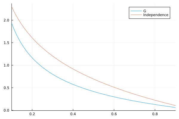

The 𝒲 alias stands for WiliamsonGenerator. To stress the generality of the approach, remark that any positive distribution is allowed, including discrete ones:

using Distributions
using Copulas: 𝒲, ϕ⁻¹
using Plots
G1 = 𝒲(Binomial(10,0.3), 2)
G2 = 𝒲(Binomial(10,0.3), 3)
plot(x -> ϕ⁻¹(G1,x), xlims=(0.1,0.9), label="G1")
plot!(x -> ϕ⁻¹(G2,x), xlims=(0.1,0.9), label="G2")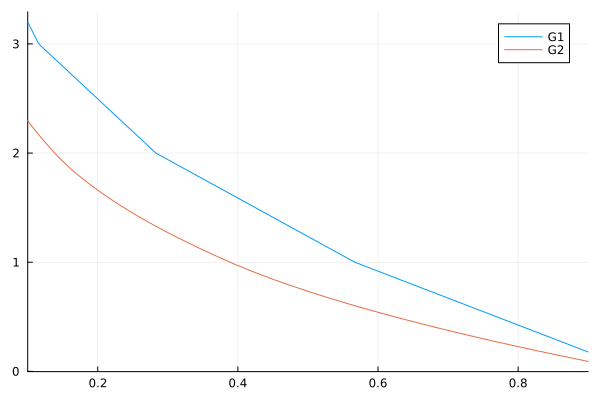

As obvious from the definition of the Williamson transform, using a discrete distribution produces piecewise-linear generators, where the number of pieces is dependent on the order of the transformation.

Archimedean Copulas

Let's first define formally archimedean copulas:

Definition: Archimedean copula

If $\varphi$ is a $d$-monotonous Archimedean generator, then the function

$$C(\mathit{u})=\varphi (\sum _{i=1}^d{\varphi }^{-1}(u_i))$$

is a copula.

There are a few archimedean generators that are worth noting since they correspond to known archimedean copulas families:

• IndependentCopula: $\varphi (t)=e^{-t}\text{ generates }\mathrm{\Pi }$.

• ClaytonGenerator: ${\varphi }_{\theta }(t)={(1+t\theta )}^{-{\theta }^{-1}}$ generates the $\mathrm{Clayton}(\theta )$ copula.

• GumbelGenerator: ${\varphi }_{\theta }(t)=\exp \{-t^{{\theta }^{-1}}\}$ generates the $\mathrm{Gumbel}(\theta )$ copula.

• FrankGenerator: ${\varphi }_{\theta }(t)=-{\theta }^{-1}\ln (1+e^{-t-\theta }-e^{-t})$ generates the $\mathrm{Franck}(\theta )$ copula.

There are a lot of others implemented in the package, see our large list of implemented archimedean generator.

Archimedean copulas have a nice decomposition, called the Radial-simplex decomposition, developed in [14, 29]:

Property: Radial-simplex decomposition

A $d$-variate random vector $\mathit{U}$ following an Archimedean copula with generator $\varphi$ can be decomposed into

$$\mathit{U}=\varphi .(\mathit{S}R),$$

where $\mathit{S}$ is uniform on the $d$-variate simplex and $R$ is a non-negative random variable, independent form $\mathit{S}$, defined as the inverse Williamson $d$-transform of $\varphi$.

This is why 𝒲₋₁(G::Generator,d) is such an important function in the API: it allows to generator the radial part and sample the Archimedean copula. You may call this function directly to see what distribution will be used:

using Copulas: 𝒲₋₁, FrankGenerator
𝒲₋₁(FrankGenerator(7), 3)

Copulas.WilliamsonFromFrailty{Copulas.Logarithmic{Float64}, 3}(
frailty_dist: Copulas.Logarithmic{Float64}(α=0.9990881180344455, h=-7.0)
)

For the Frank Copula, as for many classic copulas, the distribution used is known. We pull some of them from Distributions.jl but implement a few more, as this Logarithmic one. Another useful example are negatively-dependent Clayton copulas:

using Copulas: 𝒲₋₁, ClaytonGenerator
𝒲₋₁(ClaytonGenerator(-0.2), 3)

Copulas.ClaytonWilliamsonDistribution{Float64}(θ=-0.2, d=3)

for which the corresponding distribution is known but has no particular name, thus we implemented it under the ClaytonWilliamsonDistribution name.

Info: Frailty decomposition for completely monotone generators

It is well-known that completely monotone generators are Laplace transforms of non-negative random variables. This gives rise to another decomposition in [30]:

Property: Frailty decomposition

When $\varphi$ is completely monotone, it is the Laplace transform of a non-negative random variable $W$ such that

$$\mathit{U}=\varphi (\mathit{Y}/W),$$

where $\mathit{Y}$ is a vector of independent and identically distributed (i.i.d.) exponential distributions.

The link between the distribution of $R$ and the distribution of $W$ can be made explicit. We provide the WilliamsonFromFrailty() constructor to build the distribution of $R$ from the distribution of $W$ and return the corresponding WilliamsonGenerator from the frailty distribution itself. The corresponding φ is simply the Laplace transform of $W$. This is another way to construct new Archimedean copulas !

We use this fraily approach for several generators, since sometimes it is faster, including e.g. the Clayton one with positive dependence:

using Copulas: 𝒲₋₁, ClaytonGenerator
𝒲₋₁(ClaytonGenerator(10), 3)

Copulas.WilliamsonFromFrailty{Distributions.Gamma{Float64}, 3}(
frailty_dist: Distributions.Gamma{Float64}(α=0.1, θ=10.0)
)

:::

Copulas.ArchimedeanCopula Type

ArchimedeanCopula{d, TG}

Fields: - G::TG : the generator <: Generator.

Constructor:

ArchimedeanCopula(d::Int,G::Generator)

For some Archimedean Generator G::Generator and some dimenson d, this class models the archimedean copula which has this generator. The constructor checks for validity by ensuring that max_monotony(G) ≥ d. The $d$-variate archimedean copula with generator $\varphi$ writes:

$$C(\mathbf{u})={\varphi }^{-1}(\sum _{i=1}^d\varphi (u_i))$$

The default sampling method is the Radial-simplex decomposition using the Williamson transformation of $\varphi$.

There exists several known parametric generators that are implement in the package. For every NamedGenerator <: Generator implemented in the package, we provide a type alias ``NamedCopula{d,...} = ArchimedeanCopula{d,NamedGenerator{...}}` to be able to manipulate the classic archimedean copulas without too much hassle for known and usefull special cases.

A generic archimedean copula can be constructed as follows:

struct MyGenerator <: Generator end
ϕ(G::MyGenerator,t) = exp(-t) # your archimedean generator, can be any d-monotonous function.
max_monotony(G::MyGenerator) = Inf # could depend on generators parameters.
C = ArchimedeanCopula(d,MyGenerator())

The obtained model can be used as follows:

spl = rand(C,1000)   # sampling
cdf(C,spl)           # cdf
pdf(C,spl)           # pdf
loglikelihood(C,spl) # llh

Bonus: If you know the Williamson d-transform of your generator and not your generator itself, you may take a look at WilliamsonGenerator that implements them. If you rather know the frailty distribution, take a look at WilliamsonFromFrailty.

References:

• [28] Williamson, R. E. (1956). Multiply monotone functions and their Laplace transforms. Duke Math. J. 23 189–207. MR0077581

• [14] McNeil, A. J., & Nešlehová, J. (2009). Multivariate Archimedean copulas, d-monotone functions and ℓ 1-norm symmetric distributions.

source

Conditionals and distortions

Let $C(\mathit{u})=\varphi (\sum _{k=1}^d{\varphi }^{-1}(u_k))$ be a $d$-variate Archimedean copula with generator $\varphi$.

• Conditioning on a subset $J\subset \{1,\dots ,d\}$ with $m=|J|$ and defining $S_J=\sum _{j\in J}{\varphi }^{-1}(u_j)$, the conditional copula of the remaining coordinates $I=\{1,\dots ,d\}\setminus J$ given $U_J={\mathit{u}}_J$ is again Archimedean with generator ${\varphi }_{|J}(t;{\mathit{u}}_J)=\frac{{\varphi }^{(m)}(t+S_J)}{{\varphi }^{(m)}(S_J)},$ provided the $m$-th derivative exists and ${\varphi }^{(m)}(S_J)\ne 0$.

• The corresponding univariate conditional distortion for coordinate $i\in I$ is $H_{i|J}(u\mid {\mathit{u}}_J)=\frac{{\varphi }^{(m)}({\varphi }^{-1}(u)+S_J)}{{\varphi }^{(m)}(S_J)}\in [0,1].$

In particular, in the bivariate case ($d=2$, $J=\{2\}$) one recovers the familiar closed form

$$H_{1|2}(u\mid v)=\frac{{\varphi }^{\prime }({\varphi }^{-1}(u)+{\varphi }^{-1}(v))}{{\varphi }^{\prime }({\varphi }^{-1}(v))}.$$

These expressions are used in the implementation to provide fast paths for condition(::ArchimedeanCopula, ...) and for conditional distortions on the copula scale.

Quick visual comparison (bivariate)

using Copulas, Plots, Distributions
using Plots.PlotMeasures
Cs = (
    ClaytonCopula(2, 2.0),
    GumbelCopula(2, 1.6),
    FrankCopula(2, 8.0),
    IndependentCopula(2),
)
plot(plot.(Cs)..., layout=(2,2))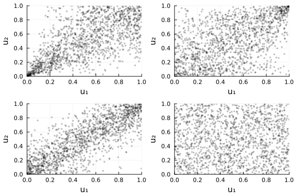

Conditional distortions (uniform scale)

using StatsBase
C = ClaytonCopula(2, 2.0)
u2 = 0.3
D = condition(C, 2, u2)
ts = range(0.0, 1.0; length=401)
plot(ts, cdf.(Ref(D), ts); label="H_{1|2}(u|$u2)", xlabel="u", ylabel="CDF",
    title="Conditional distortion for Clayton(θ=2)")
αs = rand(2000); us = Distributions.quantile.(Ref(D), αs)
EC = ecdf(us)
plot!(ts, EC.(ts); seriestype=:steppost, alpha=0.5, color=:black, label="empirical")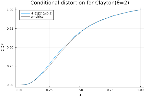

Liouville Copulas

Todo: Not merged yet !

Liouville copulas are coming in this PR : https://github.com/lrnv/Copulas.jl/pull/83, but the work is not finished.

Archimedean copulas have been widely used in the literature due to their nice decomposition properties and easy parametrization. The interested reader can refer to the extensive literature [31–37, 37–40] on Archimedean copulas, their nesting extensions and most importantly their estimation.

One major drawback of the Archimedean family is that these copulas have exchangeable marginals (i.e., $C(\mathit{u})=C(p(\mathit{u}))$ for any permutation $p(\mathit{u})$ of $u_1,...,u_d$): the dependence structure is symmetric, which might not be desirable. However, from the Radial-simplex expression, we can extrapolate and take for $\mathit{S}$ a non-uniform distribution on the simplex.

Liouville's copulas share many properties with Archimedean copulas, but are not exchangeable anymore. This is an easy way to produce non-exchangeable dependence structures. See [23] for a practical use of this property.

Note that Dirichlet distributions are constructed as $\mathit{S}=\frac{\mathit{G}}{⟨\mathbf{1},\mathit{G}⟩}$, where $\mathit{G}$ is a vector of independent Gamma distributions with unit scale (and potentially different shapes: taking all shapes equal yields the Archimedean case).

Available models

WilliamsonGenerator

Copulas.WilliamsonGenerator Type

WilliamsonGenerator{TX, d} (alias 𝒲{TX, d})

Fields:

• X::TX – a random variable that represents its Williamson d-transform

The type parameter d::Int is the dimension of the transformation.

Constructor

WilliamsonGenerator(X::Distributions.UnivariateDistribution, d)
𝒲(X::Distributions.UnivariateDistribution,d)
WilliamsonGenerator(atoms::AbstractVector, weights::AbstractVector, d)
𝒲(atoms::AbstractVector, weights::AbstractVector, d)

The WilliamsonGenerator (alias 𝒲) allows to construct a d-monotonous archimedean generator from a positive random variable X::Distributions.UnivariateDistribution. The transformation, which is called the inverse Williamson transformation, is implemented fully generically in the package.

For a univariate non-negative random variable $X$, with cumulative distribution function $F$ and an integer $d\ge 2$, the Williamson-d-transform of $X$ is the real function supported on $[0,\mathrm{\infty }[$ given by:

$$\varphi (t)={𝒲}_d(X)(t)={\int }_t^{\mathrm{\infty }}{(1-\frac{t}{x})}^{d-1}dF(x)=\mathbb{E}((1-\frac{t}{X}{)}_{+}^{d-1}){\mathbb{1}}_{t>0}+(1-F(0)){\mathbb{1}}_{t<0}$$

This function has several properties:

• We have that $\varphi (0)=1$ and $\varphi (Inf)=0$

• $\varphi$ is $d-2$ times derivable, and the signs of its derivatives alternates : $\mathrm{\forall }k\in 0,...,d-2,(-1{)}^k{\varphi }^{(k)}\ge 0$.

• ${\varphi }^{(d-2)}$ is convex.

These properties makes this function what is called a d-monotone archimedean generator, able to generate archimedean copulas in dimensions up to $d$. Our implementation provides this through the Generator interface: the function $\varphi$ can be accessed by

G = WilliamsonGenerator(X, d)
ϕ(G,t)

Note that you'll always have:

max_monotony(WilliamsonGenerator(X,d)) === d

Special case (finite-support discrete X)

• If X isa Distributions.DiscreteUnivariateDistribution and support(X) is finite, or if you pass directly atoms and weights to the constructor, the produced generator is piecewise-polynomial ϕ(t) = ∑_j w_j · (1 − t/r_j)_+^(d−1) matching the Williamson transform of a discrete radial law. It has specialized methods.

• For infinite-support discrete distributions or when the support is not accessible as a finite iterable, the standard WilliamsonGenerator is constructed.

References:

• [28] Williamson, R. E. (1956). Multiply monotone functions and their Laplace transforms. Duke Math. J. 23 189–207. MR0077581

• [14] McNeil, Alexander J., and Johanna Nešlehová. "Multivariate Archimedean copulas, d-monotone functions and ℓ 1-norm symmetric distributions." (2009): 3059-3097.

source

EmpiricalGenerator

Copulas.EmpiricalGenerator Function

EmpiricalGenerator(u::AbstractMatrix)

Nonparametric Archimedean generator fit via inversion of the empirical Kendall distribution.

This function returns a WilliamsonGenerator{TX, d} whose underlying distribution TX is a Distributions.DiscreteNonParametric, rather than a separate struct. The returned object still implements all optimized methods (ϕ, derivatives, inverses) via specialized dispatch on WilliamsonGenerator{<:DiscreteNonParametric}.

Usage

G = EmpiricalGenerator(u)

where u::AbstractMatrix is a d×n matrix of observations (already on copula or pseudo scale).

Notes

• The recovered discrete radial support is rescaled so its largest atom equals 1 (scale is not identifiable).

• We keep the old documentation entry point for backward compatibility; existing code that relied on the EmpiricalGenerator type should instead treat the result as a Generator.

References

• [41]

• [42]

• [36] Genest, Neslehova and Ziegel (2011), Inference in Multivariate Archimedean Copula Models

source

TiltedGenerator

Copulas.TiltedGenerator Type

TiltedGenerator(G, p, sJ)

Archimedean generator tilted by conditioning on p components fixed at values with cumulative generator sum sJ = ∑ ϕ⁻¹(u_j). It defines

ϕ_tilt(t) = ϕ^{(p)}(sJ + t) / ϕ^{(p)}(sJ)

and higher derivatives accordingly:

ϕ_tilt^{(k)}(t) = ϕ^{(k+p)}(sJ + t) / ϕ^{(p)}(sJ)

which yields the conditional copula within the Archimedean family for the remaining d-p variables. You will get a TiltedGenerator if you condition() an archimedean copula.

source

FrailtyGenerator

Copulas.FrailtyGenerator Type

FrailtyGenerator<:AbstractFrailtyGenerator<:Generator

methods: - frailty(::FrailtyGenerator) gives the frailty - ϕ and the rest of generators are automatically defined from the frailty.

Constructor

FrailtyGenerator(D)

A Frailty generator can be defined by a positive random variable that happens to have a mgf() function to compute its moment generating function. The generator is simply:

$$\varphi (t)=mgf(frailty(G),-t)$$

https://www.uni-ulm.de/fileadmin/website_uni_ulm/mawi.inst.zawa/forschung/2009-08-16_hofert.pdf

References:

• [43] M. Hoffert (2009). Efficiently sampling Archimedean copulas

source

ClaytonGenerator

Copulas.ClaytonGenerator Type

ClaytonGenerator{T}, ClaytonCopula{d, T}

Fields:

• θ::Real - parameter

Constructor

ClaytonGenerator(θ)
ClaytonCopula(d, θ)

The Clayton copula in dimension $d$ is parameterized by $\theta \in [-1/(d-1),\mathrm{\infty })$ (with the independence case as the limit $\theta \to 0$). It is an Archimedean copula with generator

$$\varphi (t)={(1+\theta t)}^{-1/\theta }$$

with the continuous extension $\varphi (t)=e^{-t}$ at $\theta =0$.

Special cases (for the copula in dimension $d$):

• When $\theta =-1/(d-1)$, it is the WCopula (Lower Fréchet–Hoeffding bound)

• When $\theta \to 0$, it is the IndependentCopula

• When $\theta \to \mathrm{\infty }$, it is the MCopula (Upper Fréchet–Hoeffding bound)

References:

• [3] Nelsen, Roger B. An introduction to copulas. Springer, 2006.

source

FrankGenerator

Copulas.FrankGenerator Type

FrankGenerator{T}, FrankCopula{d, T}

Fields:

• θ::Real - parameter

Constructor

FrankGenerator(θ)
FrankCopula(d,θ)

The Frank copula in dimension $d$ is parameterized by $\theta \in (-\mathrm{\infty },\mathrm{\infty })$ (with independence as the limit $\theta \to 0$). It is an Archimedean copula with generator

$$\varphi (t)=-\frac{1}{\theta }\log (1-(1-e^{-\theta })e^{-t}).$$

Special cases:

• When $\theta \to -\mathrm{\infty }$, it is the WCopula (Lower Fréchet–Hoeffding bound)

• When $\theta \to 0$, it is the IndependentCopula

• When $\theta \to \mathrm{\infty }$, it is the MCopula (Upper Fréchet–Hoeffding bound)

References:

• [3] Nelsen, Roger B. An introduction to copulas. Springer, 2006.

source

GumbelGenerator

Copulas.GumbelGenerator Type

GumbelGenerator{T}, GumbelCopula{d, T}

Fields:

• θ::Real - parameter

Constructor

GumbelGenerator(θ)
GumbelCopula(d,θ)

The Gumbel copula in dimension $d$ is parameterized by $\theta \in [1,\mathrm{\infty })$. It is an Archimedean copula with generator :

$$\varphi (t)=\exp (-t^{1/\theta }).$$

It has a few special cases:

• When θ = 1, it is the IndependentCopula

• When θ → ∞, it is the MCopula (Upper Fréchet–Hoeffding bound)

References:

• [3] Nelsen, Roger B. An introduction to copulas. Springer, 2006.

source

AMHGenerator

Copulas.AMHGenerator Type

AMHGenerator{T}, AMHCopula{d, T}

Fields:

• θ::Real - parameter

Constructors:

AMHGenerator(θ)  # Constructs the generator. 
AMHCopula(d,θ)   # Construct the copula

The AMH Copula in dimension d is parameterized by θ ∈ [-1,1). It is an Archimedean copula with generator:

$$\varphi (t)=1-\frac{1-\theta }{e^{-t}-\theta }.$$

Special cases:

• When θ = 0, it collapses to independence.

References:

• [3] Nelsen, Roger B. An introduction to copulas. Springer, 2006.

source

JoeGenerator

Copulas.JoeGenerator Type

JoeGenerator{T}, JoeCopula{d, T}

Fields:

• θ::Real - parameter

Constructor

JoeGenerator(θ)
JoeCopula(d,θ)

The Joe copula in dimension $d$ is parameterized by $\theta \in [1,\mathrm{\infty })$. It is an Archimedean copula with generator:

$$\varphi (t)=1-(1-e^{-t}{)}^{1/\theta }.$$

It has a few special cases:

• When θ = 1, it is the IndependentCopula

• When θ = ∞, it is the MCopula (Upper Fréchet–Hoeffding bound)

References:

• [3] Nelsen, Roger B. An introduction to copulas. Springer, 2006.

source

GumbelBarnettGenerator

Copulas.GumbelBarnettGenerator Type

GumbelBarnettGenerator{T}, GumbelBarnettCopula{d, T}

Fields:

• θ::Real - parameter

Constructor

GumbelBarnettGenerator(θ)
GumbelBarnettCopula(d,θ)

The Gumbel-Barnett copula is an archimdean copula with generator:

$$\varphi (t)=\exp ({\theta }^{-1}(1-e^t)),0\le \theta \le 1.$$

Special cases:

• When θ = 0, it is the IndependentCopula

References:

• [4] Joe, H. (2014). Dependence modeling with copulas. CRC press, Page.437

• [3] Nelsen, Roger B. An introduction to copulas. Springer, 2006.

source

InvGaussianGenerator

Copulas.InvGaussianGenerator Type

InvGaussianGenerator{T}, InvGaussianCopula{d, T}

Fields:

• θ::Real - parameter

Constructor

InvGaussianGenerator(θ)
InvGaussianCopula(d,θ)

The Inverse Gaussian copula in dimension $d$ is parameterized by $\theta \in [0,\mathrm{\infty })$. It is an Archimedean copula with generator:

$$\varphi (t)=\exp \left(\frac{1-\sqrt{1+2{\theta }^{2}t}}{\theta }\right).$$

More details about Inverse Gaussian Archimedean copula are found in :

Mai, Jan-Frederik, and Matthias Scherer. Simulating copulas: stochastic models, sampling algorithms, and applications. Vol. 6. # N/A, 2017. Page 74.

Special cases:

• When θ = 0, it is the IndependentCopula

References:

• [3] Nelsen, Roger B. An introduction to copulas. Springer, 2006.

source

BB1Generator

Copulas.BB1Generator Type

BB1Generator{T}, BB1Copula{d, T}

Fields:

• θ::Real - parameter

• δ::Real - parameter

Constructor

BB1Generator(θ, δ)
BB1Copula(d, θ, δ)

The BB1 copula is parameterized by $\theta \in (0,\mathrm{\infty })$ and $\delta \in [1,\mathrm{\infty })$. It is an Archimedean copula with generator:

$$\varphi (t)=(1+t^{1/\delta }{)}^{-1/\theta },$$

Special cases:

• When δ = 1, it is the ClaytonCopula with parameter $\theta$.

References:

• [4] Joe, H. (2014). Dependence modeling with copulas. CRC press, Page.190-192

source

BB2Generator

Copulas.BB2Generator Type

BB2Generator{T}, BB2Copula{d, T}

Fields:

• θ::Real - parameter

• δ::Real - parameter

Constructor

BB2Generator(θ, δ)
BB2Copula(d, θ, δ)

The BB2 copula has parameters $\theta ,\delta \in (0,\mathrm{\infty })$. It is an Archimedean copula with generator:

$$\varphi (t)=[1+{\delta }^{-1}log(1+t){]}^{-\frac{1}{\theta }},$$

References:

• [4] Joe, H. (2014). Dependence modeling with copulas. CRC press, Page.193-194

source

BB3Generator

Copulas.BB3Generator Type

BB3Generator{T}, BB3Copula{d, T}

Fields:

• θ::Real - parameter

• δ::Real - parameter

Constructor

BB3Generator(θ, δ)
BB3Copula(d, θ, δ)

The BB3 copula has parameters $\theta \in [1,\mathrm{\infty })$ and $\delta \in (0,\mathrm{\infty })$. It is an Archimedean copula with generator:

$$\varphi (t)=\exp (-[{\delta }^{-1}\log (1+t){]}^{\frac{1}{\theta }}),$$

References:

• [4] Joe, H. (2014). Dependence modeling with copulas. CRC press, Page.195-196

source

BB6Generator

Copulas.BB6Generator Type

BB6Generator{T}, BB6Copula{d, T}

Fields:

• θ::Real - parameter

• δ::Real - parameter

Constructor

BB6Generator(θ, δ)
BB6Copula(d, θ, δ)

The BB6 copula has parameters $\theta ,\delta \in [1,\mathrm{\infty })$. It is an Archimedean copula with generator:

$$\varphi (t)=1-[1-\exp (-t^{\frac{1}{\delta }}){]}^{\frac{1}{\theta }}$$

References:

• [4] Joe, H. (2014). Dependence modeling with copulas. CRC press, Page.200-201

source

BB7Generator

Copulas.BB7Generator Type

BB7Generator{T}, BB7Copula{d, T}

Fields:

• θ::Real - parameter

• δ::Real - parameter

Constructor

BB7Generator(θ, δ)
BB7Copula(d, θ, δ)

The BB7 copula is parameterized by $\theta \in [1,\mathrm{\infty })$ and $\delta \in (0,\mathrm{\infty })$. It is an Archimedean copula with generator:

$$\varphi (t)=1-[1-(1+t{)}^{-1/\delta }{]}^{1/\theta }.$$

References:

• [4] Joe, H. (2014). Dependence modeling with copulas. CRC press, Page.202-203

source

BB8Generator

Copulas.BB8Generator Type

BB8Generator{T}, BB8Copula{d, T}

Fields:

• ϑ::Real - parameter

• δ::Real - parameter

Constructor

BB8Generator(ϑ, δ)
BB8Copula(d, ϑ, δ)

The BB8 copula has parameters $\vartheta \in [1,\mathrm{\infty })$ and $\delta \in (0,1]$. It is an Archimedean copula with generator:

$$\varphi (t)={\delta }^{-1}[1-(1-\eta \exp (-t){)}^{\frac{1}{\vartheta }}],$$

where $\eta =1-(1-\delta {)}^{\vartheta }$.

References:

• [4] Joe, H. (2014). Dependence modeling with copulas. CRC press, Page.204-205

source

BB9Generator

Copulas.BB9Generator Type

BB9Generator{T}, BB9Copula{d, T}

Fields:

• ϑ::Real - parameter

• δ::Real - parameter

Constructor

BB9Generator(ϑ, δ)
BB9Copula(d, ϑ, δ)

The BB9 copula has parameters $\vartheta \in [1,\mathrm{\infty })$ and $\delta \in (0,\mathrm{\infty })$. It is an Archimedean copula with generator:

$$\varphi (t)=\exp (-({\delta }^{-\vartheta }+t{)}^{\frac{1}{\vartheta }}+{\delta }^{-1}),$$

References:

• [4] Joe, H. (2014). Dependence modeling with copulas. CRC press, Page.205-206

source

BB10Generator

Copulas.BB10Generator Type

BB10Generator{T}, BB10Copula{d, T}

Fields:

• θ::Real - parameter

• δ::Real - parameter

Constructor

BB10Generator(θ, δ)
BB10Copula(d, θ, δ)

The BB10 copula has parameters $\theta \in (0,\mathrm{\infty })$ and $\delta \in [0,1]$. It is an Archimedean copula with generator:

$$\varphi (t)=(\frac{1-\delta }{e^t-\delta }{)}^{1/\theta },$$

References:

• [4] Joe, H. (2014). Dependence modeling with copulas. CRC press, Page.206-207

source

References

1. R. B. Nelsen. An Introduction to Copulas. 2nd ed Edition, Springer Series in Statistics (Springer, New York, 2006).

2. H. Joe. Dependence Modeling with Copulas (CRC press, 2014).

3. A. J. McNeil and J. Nešlehová. Multivariate Archimedean Copulas, d -Monotone Functions and L1 -Norm Symmetric Distributions. The Annals of Statistics 37, 3059–3097 (2009).

4. M.-P. Côté and C. Genest. Dependence in a Background Risk Model. Journal of Multivariate Analysis 172, 28–46 (2019).

5. R. E. Williamson. On multiply monotone functions and their laplace transforms (Mathematics Division, Office of Scientific Research, US Air Force, 1955).

6. A. J. McNeil. Sampling Nested Archimedean Copulas. Journal of Statistical Computation and Simulation 78, 567–581 (2008).

7. M. Hofert, M. Mächler and A. J. McNeil. Archimedean Copulas in High Dimensions: Estimators and Numerical Challenges Motivated by Financial Applications. Journal de la Société Française de Statistique 154, 25–63 (2013).

8. M. Hofert. Sampling Nested Archimedean Copulas with Applications to CDO Pricing. Ph.D. Thesis, Universität Ulm (2010).

9. M. Hofert and D. Pham. Densities of Nested Archimedean Copulas. Journal of Multivariate Analysis 118, 37–52 (2013).

10. A. J. McNeil and J. Nešlehová. From Archimedean to Liouville Copulas. Journal of Multivariate Analysis 101, 1772–1790 (2010).

11. H. Cossette, S.-P. Gadoury, E. Marceau and I. Mtalai. Hierarchical Archimedean Copulas through Multivariate Compound Distributions. Insurance: Mathematics and Economics 76, 1–13 (2017).

12. H. Cossette, E. Marceau, I. Mtalai and D. Veilleux. Dependent Risk Models with Archimedean Copulas: A Computational Strategy Based on Common Mixtures and Applications. Insurance: Mathematics and Economics 78, 53–71 (2018).

13. C. Genest, J. Nešlehová and J. Ziegel. Inference in Multivariate Archimedean Copula Models. TEST 20, 223–256 (2011).

14. E. Di Bernardino and D. Rulliere. On Certain Transformations of Archimedean Copulas: Application to the Non-Parametric Estimation of Their Generators. Dependence Modeling 1, 1–36 (2013).

15. E. Di Bernardino and D. Rullière. On an Asymmetric Extension of Multivariate Archimedean Copulas Based on Quadratic Form. Dependence Modeling 4 (2016).

16. K. Cooray. Strictly Archimedean Copulas with Complete Association for Multivariate Dependence Based on the Clayton Family. Dependence Modeling 6, 1–18 (2018).

17. J. Spreeuw. Archimedean Copulas Derived from Utility Functions. Insurance: Mathematics and Economics 59, 235–242 (2014).

18. A. J. McNeil and J. Nešlehová. Multivariate Archimedean copulas, $d$-monotone functions and ${\ell }_1$-norm symmetric distributions. Annals of Statistics 37, 3059–3097 (2009).

19. R. E. Williamson. Multiply monotone functions and their Laplace transforms. Duke Mathematical Journal 23, 189–207 (1956).

20. M. Hofert. Efficiently sampling Archimedean copulas (2009).

---

1. This bijection is to be taken carefuly: the bijection is between random variables with unit scales and generators with common value at 1, sicne on both rescaling does not change the underlying copula. ↩︎