Conditioning and Subsetting

Conditioning

This page introduces conditional distributions under a copula model and shows how to construct them programmatically using condition. The same interface works either on the uniform scale (copula only) or on the original scale (via SklarDist).

Overview

Take a $d$-variate copula $C$ and partition the coordinates into conditioned indices $J$ and remaining indices $I$. In the regular case, where the required derivatives exist and the conditioning marginal has a finite, positive density, the conditional CDF on the uniform scale is given almost everywhere by

$$H_{I\mid J}({\mathbf{u}}_I\mid {\mathbf{u}}_J):=\frac{{\partial }^{p}C({\mathbf{u}}_I,{\mathbf{u}}_J)}{\partial {\mathbf{u}}_J}/\frac{{\partial }^{p}C({\mathbf{1}}_I,{\mathbf{u}}_J)}{\partial {\mathbf{u}}_J},$$

which defines a distribution on $[0,1{]}^{|I|}$ under these assumptions. This derivative ratio is not a universal construction at singular points or where the denominator vanishes. Supported singular models may instead use specialized conditional distributions, including atoms. A conditional law is determined only almost everywhere with respect to the conditioning marginal; values outside that set require a choice of version.

Each conditional marginal can be expressed as a “distortion” $H_{i|J}(·|u_J)$, a distribution on $[0,1]$ that need not be uniform. Under the same regularity assumptions, its CDF is

$$H_{i\mid J}(u\mid {\mathbf{u}}_J):=\frac{{\partial }^{p}C({\mathbf{u}}^{(i)}(u_I),{\mathbf{u}}_J)}{\partial {\mathbf{u}}_J}/\frac{{\partial }^{p}C(\mathbf{1},{\mathbf{u}}_J)}{\partial {\mathbf{u}}_J},$$

where ${\mathbf{u}}^{(i)}(u_I)$ has coordinate u at index i and 1 elsewhere in I.

For continuous, invertible conditioning margins of X = SklarDist(C, (X_1,…,X_D)), conditioning on $x_J$ can be transferred to $u_J=(F_j(x_j){)}_{j\in J}$ and expressed on the remaining marginal scales:

$$F_{X_i\mid X_J}(x\mid {\mathbf{x}}_J)=H_{i\mid J}(F_i(x)\mid {\mathbf{u}}_J).$$

Conditioning on an interval

A conditioning event is not always a point. A stress such as "$U_3$ in its bottom decile", $U_3\in [0,0.1]$, or a joint box on two or three coordinates, asks for the law of the other coordinates given an event of positive probability. Partition the conditioned coordinates into point coordinates $P$ with values ${\mathbf{u}}_P$ and interval coordinates $B$ with box $\prod _{j\in B}[a_j,b_j]$, with $I$ free. The conditional CDF of ${\mathbf{U}}_I$ is the inclusion–exclusion sum over the $2^{|B|}$ corners of the box of the same partial derivatives,

$$H_{I\mid P,B}({\mathbf{u}}_I)=\frac{\sum _{c\in \mathrm{corners}(B)}\mathrm{sgn}(c){\partial }_{{\mathbf{u}}_P}C({\mathbf{u}}_I,{\mathbf{u}}_P,c)}{\sum _{c\in \mathrm{corners}(B)}\mathrm{sgn}(c){\partial }_{{\mathbf{u}}_P}C({\mathbf{1}}_I,{\mathbf{u}}_P,c)},\mathrm{sgn}(c)=(-1{)}^{\mathrm{\#}\{j:c_j=a_j\}}.$$

With $P=\mathrm{\varnothing }$ both sides are C-volumes, the objects measure computes; with $B=\mathrm{\varnothing }$ it is the point formula above. The denominator is a probability rather than a density, so the interval form is defined wherever the box has positive probability and needs no choice of version. The conditional density on ${\mathbf{u}}_I$ is the $|I|$-th mixed partial of the same sum, so logpdf, quantile and sequential sampling all reduce to one primitive. Substituting the midpoint of an interval into the point conditional is not a substitute: on ClaytonCopula(3, 2.0) with $U_3\in [0,0.1]$, the CDF of $U_1\mid U_3=0.05$ and the CDF of $U_1\mid U_3\in [0,0.1]$ differ by more than $0.05$.

The entry point is the four-argument form of condition:

• condition(C::Copula, js, lo_js, hi_js) conditions on $U_{j_k}\in [{\mathrm{lo}}_k,{\mathrm{hi}}_k]$ for each $k$. A coordinate with lo == hi is conditioned on that point, so condition(C, js, u, u) is condition(C, js, u) and one call may mix fixed values with intervals. Bounds must satisfy $0\le \mathrm{lo}\le \mathrm{hi}\le 1$ and a box of zero probability throws an ArgumentError.

• condition(X::SklarDist, js, xlo_js, xhi_js) takes the intervals on the original scale and maps them through the margins.

The return shape follows the point form: a univariate distribution when one coordinate is free, otherwise a multivariate distribution of the conditional copula and the conditional margins.

Discrete margins

Observing a discrete margin $X_j=x_j$ of a SklarDist is the latent event $U_j\in (F_j(x_j^{-}),F_j(x_j)]$, an interval, not the point $F_j(x_j)$. condition(X, js, x_js) therefore conditions each discrete coordinate on its interval and each continuous one on its point, in the one call; a discrete observation of zero probability throws. The same latent interval gives the probability mass of a SklarDist with atoms, so pdf and logpdf are the mixed derivative in the continuous coordinates and the finite difference over the discrete ones, times the continuous marginal densities only. Conditioning a model whose free margin is discrete yields a distribution whose pdf is the conditional probability mass of the atom.

The exact discrete likelihood costs $2^k$ copula CDF evaluations for $k$ discrete margins, which is the mathematics rather than the implementation; a high-dimensional discrete model calls for a simulated likelihood.

The Rosenblatt transform of a discrete coordinate is not unique, since the observation is an interval of latent uniforms. rosenblatt(rng, X, x) draws the distributional transform of [ DocumenterCitations.CitationSiteNode("ruschendorf2009-cite-1")

] within that interval, the randomisation of [ DocumenterCitations.CitationSiteNode("brockwell2007-cite-1")

], and conditions every later coordinate on the interval as the discrete pair-copula constructions of [ DocumenterCitations.CitationSiteNode("panagiotelis2012-cite-1")

] do, so the output is independent uniform when the model is correct; inverse_rosenblatt(X, s) needs no randomness. This is the convention of vinecopulib's rosenblatt(…, randomize_discrete = TRUE). The probability mass of a SklarDist with atoms is the one [ DocumenterCitations.CitationSiteNode("genest2007-cite-1")

] write down.

A copula of the conditional vector is denoted $C_{I|J}(·|u_J)$; it need not be unique when conditional margins have atoms. The public entry point is condition:

• condition(C::Copula, js, u_js) returns the conditional distribution of the remaining U_I on the original copula coordinate scale for I = setdiff(1:D, js). Its conditional margins need not be uniform. If length(I) == 1, the result is a univariate distribution supported on [0, 1]; otherwise it is a multivariate distribution implementing the usualDistributions.jl` interface.

• condition(X::SklarDist, js, x_js) returns the conditional distribution on the original scale by pushing forward each distortion through the corresponding marginal.

• Known parametric families may use specialized representations, but their concrete types are implementation details and do not change this contract.

Missing fast-paths?

If you find a conditional that should admit a faster closed-form or semi-analytic path but currently falls back to the generic construction, please open an issue, we’ll happily implement it 😃

Examples

Let us visualize a given univariate distortion:

using Copulas, Distributions, Plots, StatsBase
C = ClaytonCopula(2, 1.5)
D = condition(C, 2, 0.3)  # distortion for U₁ | U₂ = 0.3
ts = range(0.0, 1.0; length=401)
plt = plot(ts, cdf.(Ref(D), ts);
          xlabel="u", ylabel="H_{1|2}(u | 0.3)",
          title="Conditional CDF on the uniform scale",
          legend=false)
plt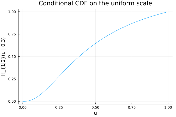

Confirm the result by overlaying the empirical cdf of a sample:

N = 2000
αs = rand(N)
us = Distributions.quantile.(Ref(D), αs)
ECDF = ecdf(us)
plot!(ts, ECDF.(ts); seriestype=:steppost, label="empirical", alpha=0.6, color=:black)
plot!(ts, cdf.(Ref(D), ts); label="analytic", color=:blue)
plt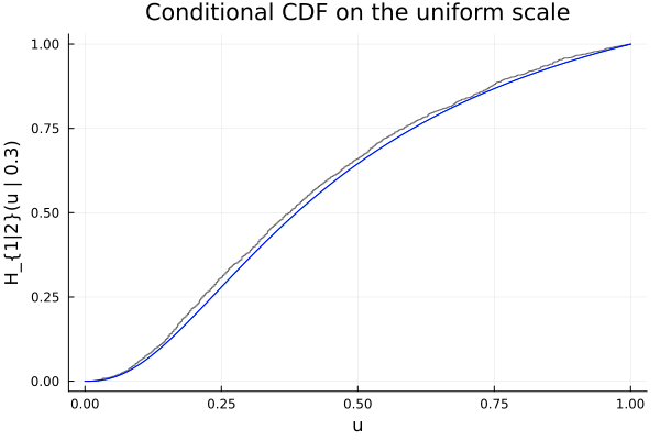

The same thing can be done on marginal scales using SklarDist:

C = ClaytonCopula(2, 1.5)
X = SklarDist(C, (Normal(), Normal()))
X1_given_X2 = condition(X, 2, 0.0) # distribution of X₁ | X₂ = 0.0
cdf(X1_given_X2, 1.0), quantile(X1_given_X2, 0.95)

(0.847233793031909, 1.5990201973152862)

xs = rand(X1_given_X2, 2000)
Fx = ecdf(xs)
xs_grid = range(quantile(X1_given_X2, 0.001), quantile(X1_given_X2, 0.999); length=401)
plot(xs_grid, Distributions.cdf.(Ref(X1_given_X2), xs_grid);
  xlabel="x", ylabel="F_{X₁|X₂}(x|0)", title="Original-scale conditional CDF", label="analytic")
plot!(xs_grid, Fx.(xs_grid); seriestype=:steppost, label="empirical", alpha=0.6, color=:black)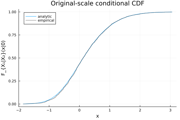

When conditioning on less than $D-1$ dimensions, we obtain a multivariate object, usually a SklarDist:

H = condition(ClaytonCopula(4, 4.2), (2, 3), (0.25, 0.8))

SklarDist{ArchimedeanCopula{2, Copulas.TiltedGenerator{Copulas.ClaytonGenerator{Float64}, Float64}}, Tuple{Copulas.ArchimedeanDistortion{Copulas.ClaytonGenerator{Float64}, Float64}, Copulas.ArchimedeanDistortion{Copulas.ClaytonGenerator{Float64}, Float64}}}(
C: ArchimedeanCopula{2, Copulas.TiltedGenerator{Copulas.ClaytonGenerator{Float64}, Float64}}(Copulas.ClaytonGenerator{Float64}(4.2), 2, 80.55877526114391)
m: (Copulas.ArchimedeanDistortion{Copulas.ClaytonGenerator{Float64}, Float64}(
G: Copulas.ClaytonGenerator{Float64}(4.2)
p: 2
sJ: 80.55877526114391
den: 1.127668472157615e-5
)
, Copulas.ArchimedeanDistortion{Copulas.ClaytonGenerator{Float64}, Float64}(
G: Copulas.ClaytonGenerator{Float64}(4.2)
p: 2
sJ: 80.55877526114391
den: 1.127668472157615e-5
)
)
)

plot(H)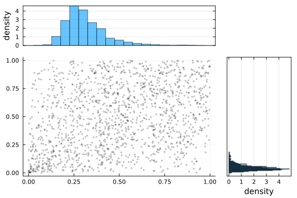

Conditioning on an interval uses the four-argument form. Here is the conditional CDF of $U_1$ given $U_3$ in its bottom decile, next to the point conditional at the midpoint of that decile:

C = ClaytonCopula(3, 2.0)
D_box = condition(C, (2, 3), (0.0, 0.0), (1.0, 0.1))   # U₁ | U₃ ∈ [0, 0.1]
D_mid = condition(C, (2, 3), (1.0, 0.05))              # U₁ | U₂ = 1, U₃ = 0.05
plot(ts, cdf.(Ref(D_box), ts); label="U₃ ∈ [0, 0.1]", xlabel="u", ylabel="H(u)")
plot!(ts, cdf.(Ref(D_mid), ts); label="U₃ = 0.05")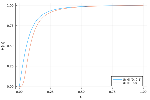

A mixed event fixes one coordinate and boxes another, and a SklarDist with a discrete margin conditions that margin on the latent interval of the observation:

condition(C, (2, 3), (0.7, 0.0), (0.7, 0.1))            # U₁ | U₂ = 0.7, U₃ ∈ [0, 0.1]
X = SklarDist(ClaytonCopula(2, 2.0), (Normal(), Poisson(3.0)))
X1_given_X2 = condition(X, 2, 2)                        # X₁ | X₂ = 2, i.e. U₂ ∈ (F(1), F(2)]
cdf(X1_given_X2, 0.0), pdf(X, [0.0, 2])

(0.6831574759280874, 0.10560989034106077)

Relation to the conditional copula

The conditional copula $C_{I|J}(·|u_J)$ is the copula of the conditional distribution $H_{I|J}(·|u_J)$. For a multivariate result, the copula and margins are available through the public params interface:

first(params(H))

ArchimedeanCopula{2, Copulas.TiltedGenerator{Copulas.ClaytonGenerator{Float64}, Float64}}(Copulas.ClaytonGenerator{Float64}(4.2), 2, 80.55877526114391)

last(params(H))

(Copulas.ArchimedeanDistortion{Copulas.ClaytonGenerator{Float64}, Float64}(
G: Copulas.ClaytonGenerator{Float64}(4.2)
p: 2
sJ: 80.55877526114391
den: 1.127668472157615e-5
)
, Copulas.ArchimedeanDistortion{Copulas.ClaytonGenerator{Float64}, Float64}(
G: Copulas.ClaytonGenerator{Float64}(4.2)
p: 2
sJ: 80.55877526114391
den: 1.127668472157615e-5
)
)

See the canonical Public API entry for condition.

See also

• condition — reference documentation with all calling syntaxes

• SklarDist — compound distributions via Sklar’s theorem

• rosenblatt — sequential transforms (related but different)

Subsetting

Subsetting extracts the dependence structure among a subset of coordinates. Given a copula C of dimension d and an index tuple dims::NTuple{p,Int}, the function subsetdims returns a copula on those p dimensions that preserves the original dependence restricted to dims.

There are two entry points:

• subsetdims(C::Copula, dims) returns a Copula{p} (or Uniform() when p == 1).

• subsetdims(X::SklarDist, dims) returns the corresponding joint distribution with the selected copula coordinates and margins, in the requested order.

The concrete representation is family-dependent. Some families return a natural reduced-parameter form, while the generic path uses an internal delegating representation. Both implement the same public copula interface:

using Copulas, Distributions
C = GaussianCopula([1.0 0.6 0.2; 0.6 1.0 0.3; 0.2 0.3 1.0])
S = subsetdims(C, (1,3))    # 2D copula on coordinates 1 and 3
length(S), cdf(S, [0.5, 0.5])

(2, 0.2820806658933831)

X = SklarDist(C, (Normal(), Normal(1,2), LogNormal()))
X13 = subsetdims(X, (1,3))  # keeps marginals (Normal(), LogNormal()) and reduces the copula
length(first(params(X13))), length(last(params(X13)))

(2, 2)

The exact result type is not part of the contract. Specialized forms may provide better performance or clearer display, while every result remains usable through the same copula API.

Subsetting and conditioning commute in the obvious way: conditioning on coordinates J and then extracting a subset of the remaining coordinates is equivalent to subsetting the base copula first and then conditioning on the corresponding indices.

Examples

# Archimedean example
C = ClaytonCopula(3, 2.0)
S = subsetdims(C, (1,2))        # still a ClaytonCopula with the same parameter
rand(S, 3)                      # sample 3 points
cdf(S, [0.7, 0.9])

0.6629375642933931

# Survival example with flips remapped
base = GaussianCopula([1.0 0.7 0.2; 0.7 1.0 0.1; 0.2 0.1 1.0])
S = SurvivalCopula(base, (2,))
S13 = subsetdims(S, (1,3))      # flip on 2 drops; no flips remain
length(S13), cdf(S13, [0.5, 0.5])

(2, 0.2820806658933831)

See the canonical Public API entry for subsetdims.

Non-copula random vectors

The operations introduced on this page are not limited to copula-based models.

Extending the interface beyond copula models

Loading PartitionedDistributions.jl activates an extension that makes condition, subsetdims, rosenblatt, and inverse_rosenblatt available for compatible vector-valued distributions implementing its public marginal and conditional interfaces. The adapter completes retained coordinates with in-support marginal medians and verifies the complete point against the joint support before conditioning. See the complete interoperability example.

For example, the extension supplies the sequential transforms of a multivariate normal distribution through its marginal and conditional distributions:

using Copulas, Distributions, PartitionedDistributions

D = MvNormal(
    [0.2, -0.3, 0.7],
    [
        1.0  0.3   0.1
        0.3  1.2   0.25
        0.1  0.25  0.8
    ],
)
x = [0.1, -0.4, 1.1]

u = rosenblatt(D, x)
x_reconstructed = inverse_rosenblatt(D, u)
(u=u, reconstruction_error=maximum(abs, x_reconstructed .- x))

(u = [0.460172162722971, 0.4735133407437463, 0.6881550316809848], reconstruction_error = 5.551115123125783e-17)

More generally, the forward transform requires cdf on each successive conditional law, while the inverse also requires quantile.

The usual caveat still applies: the deterministic forward and inverse transforms are mutual inverses only when the successive conditional CDFs are continuous and invertible on their supports.

Rosenblatt transformations

Definition and usefulness

Definition: Rosenblatt transformation

The Rosenblatt transformation evaluates successive conditional CDFs of a random vector $X$. With atomless successive conditional distributions, it transforms $X$ into independent uniforms.

More formally, consider the map $R_X(x)$ defined as follows:

$$R_X(x_1,...,x_d)=(r_1=F_{X_1}(x_1),r_2=F_{X_2|X_1}(x_2|x_1),...,r_d=F_{X_d|X_1,...,X_{d-1}}(x_d|x_1,...,x_{d-1}))$$

References:

• [ DocumenterCitations.CitationSiteNode("rosenblatt1952-cite-1")

  ] Rosenblatt, M. (1952). Remarks on a multivariate transformation. Annals of Mathematical Statistics, 23(3), 470-472.

• [ DocumenterCitations.CitationSiteNode("joe2014-cite-2")

  ] Joe, H. (2014). Dependence Modeling with Copulas. CRC Press. (Section 2.10)

• [ DocumenterCitations.CitationSiteNode("mcneil2009-cite-1")

  ] McNeil, A. J., & Nešlehová, J. (2009). Multivariate Archimedean copulas, d-monotone functions and ℓ 1-norm symmetric distributions.

In certain circumstances, in particular for Archimedean copulas, this map simplifies to tractable expressions. It has a few nice properties:

• $R_X(X)\sim \mathtt{\text{Uniform(Unit Hypercube)}}$

• The forward and inverse transforms are inverses almost surely when the successive conditional CDFs are continuous and invertible on their supports.

The uniformity statement also requires atomless successive conditional laws. For atomic or singular models, the deterministic CDF transform need not produce independent uniforms and need not be invertible. Generalized conditional quantiles can still generate samples from independent uniforms when those conditional laws are implemented; this does not require a bijective forward transform. No additional randomization within CDF jumps is implicit in rosenblatt.

These two properties are leveraged in some cases to construct the inverse Rosenblatt transformations, which map random noise to proper samples from the copula. In some cases, this is the best sampling algorithm available.

For a random vector represented by a SklarDist or Copula, the public rosenblatt(X, x) and inverse_rosenblatt(X, x) operations provide the forward and inverse transforms.

See the canonical Public API entries for rosenblatt, inverse_rosenblatt.

The transforms use the same conditional laws as condition, so their availability and numerical limitations follow those of the underlying family.

Sanity check plot

You can validate that the Rosenblatt transform maps samples to independent uniforms by checking the marginal ECDFs against the 45° line.

using Copulas, Plots, StatsBase
# pick a nontrivial copula
C = ClaytonCopula(3, 1.5)

# draw samples and apply Rosenblatt transform coordinate-wise
U = rand(C, 3000)                 # size (3, N)
S = reduce(hcat, (rosenblatt(C, U[:, i]) for i in 1:size(U, 2)))  # size (3, N)

ts = range(0.0, 1.0; length=401)
layout = @layout [a b c]
plt = plot(layout=layout, size=(900, 280), legend=false)
for k in 1:3
  Ek = ecdf(S[k, :])
  plot!(plt[k], ts, Ek.(ts); seriestype=:steppost, color=:black,
      title="ECDF of $(k)", xlabel="u", ylabel="ECDF")
  plot!(plt[k], ts, ts; color=:blue, alpha=0.7)
end
plt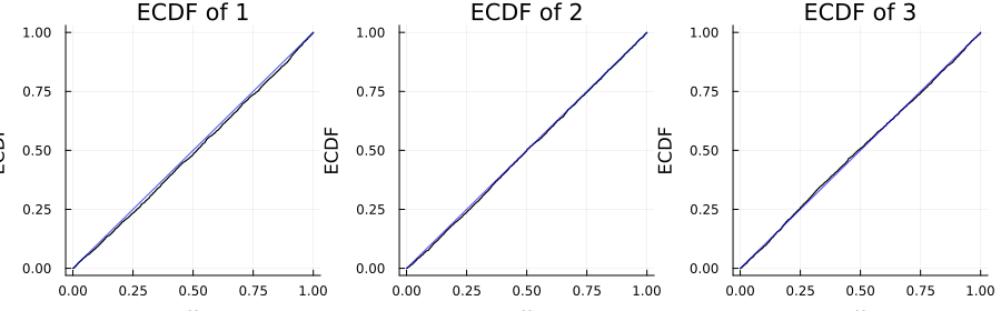

References

1. H. Joe. Dependence Modeling with Copulas (CRC press, 2014).

2. L. Rüschendorf. On the distributional transform, Sklar's theorem, and the empirical copula process. Journal of Statistical Planning and Inference 139, 3921–3927 (2009).

3. A. E. Brockwell. Universal residuals: A multivariate transformation. Statistics & Probability Letters 77, 1473–1478 (2007).

4. A. Panagiotelis, C. Czado and H. Joe. Pair copula constructions for multivariate discrete data. Journal of the American Statistical Association 107, 1063–1072 (2012).

5. C. Genest and J. Nešlehová. A primer on copulas for count data. ASTIN Bulletin 37, 475–515 (2007).

6. M. Rosenblatt. Remarks on a multivariate transformation. Annals of Mathematical Statistics 23, 470–472 (1952).

7. A. J. McNeil and J. Nešlehová. Multivariate Archimedean Copulas, $d$-Monotone Functions and ${\ell }_1$-Norm Symmetric Distributions. The Annals of Statistics 37, 3059–3097 (2009).