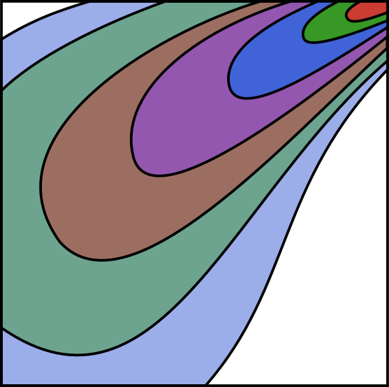
Liouville copulas

Liouville copulas replace the uniform simplex direction of an Archimedean copula by a general Dirichlet direction. Copulas.jl keeps the generator-first interface:

LiouvilleCopula{d}(G, α)

Here G is a Generator, α contains d positive real parameters, and sum(α) is the Williamson order needed by the full radial vector. The implementation accepts integer, non-integer, and mixed Dirichlet parameters.

For a general generator, ceil(sum(α)) <= max_monotony(G) is required because inversion starts at the next integer order. A generator constructed as 𝒲(R, source_order) retains R and instead accepts every sum(α) <= source_order, including values whose ceiling is larger than source_order.

Starting from a radial distribution

Suppose that the radial distribution is known at order 5.5. Any non-negative univariate distribution supported by Distributions.jl can be used, including a discrete one. An atom at one makes the order reductions especially easy to inspect.

using Copulas, Distributions, Random
using Copulas: 𝒲, 𝒲₋₁

source_radial = Dirac(1.0)
source_order = 5.5
G = 𝒲(source_radial, source_order)

α = (0.75, 1.5, 3.0)
α₀ = sum(α) # 5.25
C = LiouvilleCopula{3}(G, α)

LiouvilleCopula{3, 𝒲{Distributions.Dirac{Float64}, Float64}, Float64}(
G: 𝒲(Distributions.Dirac{Float64}(value=1.0), 5.5)
α: (0.75, 1.5, 3.0)
)

The generator contains more monotonicity than this model needs. Copulas.jl lowers its order exactly:

$$R_{5.25}=R_{5.5}B,B\sim \mathrm{Beta}(5.25,0.25).$$

This example also exercises the sharper preserved-radial path: ceil(5.25) == 6 exceeds the source order 5.5, but direct reduction from the retained radial remains exact. The same direct mechanism produces every marginal radial. Integer dispatch for a general generator, including within a mixed parameter vector, is illustrated below.

model_radial = 𝒲₋₁(G, α₀)
marginal_radials = ntuple(i -> 𝒲₋₁(G, α[i]), 3)

typeof(model_radial), typeof.(marginal_radials)

(Copulas.WilliamsonBetaProduct{Distributions.Dirac{Float64}, Distributions.Beta{Float64}, Float64}, (Copulas.WilliamsonBetaProduct{Distributions.Dirac{Float64}, Distributions.Beta{Float64}, Float64}, Copulas.WilliamsonBetaProduct{Distributions.Dirac{Float64}, Distributions.Beta{Float64}, Float64}, Copulas.WilliamsonBetaProduct{Distributions.Dirac{Float64}, Distributions.Beta{Float64}, Float64}))

The resulting object implements the usual Distributions.jl interface:

rng = Xoshiro(42)
U = rand(rng, C, 5)

C13 = subsetdims(C, (1, 3))
u13 = [0.4, 0.7]
(cdf = cdf(C13, u13), logpdf = logpdf(C13, u13), sample = U[:, 1])

(cdf = 0.22654999383250726, logpdf = -0.030945498204309807, sample = [0.13949394514011748, 0.7712489781532224, 0.4366164506825918])

Starting from an arbitrary generator

The source does not have to be a WilliamsonGenerator. For a general generator and a real target order s, Copulas.jl computes the inverse at ceil(Int, s) and multiplies it by an independent Beta(s, ceil(s) - s) variable. Existing specialized integer inverses remain in use.

G2 = Copulas.ClaytonGenerator(1.5)
α2 = (1, 0.6, 1.25)
C2 = LiouvilleCopula{3}(G2, α2)
rng = Xoshiro(42)

R3 = 𝒲₋₁(G2, 3)       # specialized integer path
Rreal = 𝒲₋₁(G2, sum(α2)) # order 2.85: R3 times Beta(2.85, 0.15)

typeof(R3), typeof(Rreal), rand(rng, C2)

(Distributions.LocationScale{Float64, Distributions.Continuous, Distributions.BetaPrime{Float64}}, Distributions.LocationScale{Float64, Distributions.Continuous, Distributions.BetaPrime{Float64}}, [0.4725908499421559, 0.797755273744378, 0.8089096298039543])

This is also why subsetting is exact and inexpensive at the model level. A subset keeps the same generator and selects the corresponding Dirichlet parameters; its smaller total order is obtained through the same Williamson reduction.

rng = Xoshiro(42)
(typeof(C13), C13.α, rand(rng, C13))

(LiouvilleCopula{2, 𝒲{Distributions.Dirac{Float64}, Float64}, Float64}, (0.75, 3.0), [0.175007720411405, 0.840092927978501])

For α = ones(d), every marginal survival function is the generator itself and the construction is exactly Archimedean. The object remains a LiouvilleCopula, while its numerical methods exploit the equivalent ArchimedeanCopula path:

G2 = Copulas.ClaytonGenerator(1.5)
LA = LiouvilleCopula{3}(G2, ones(3))
A = ArchimedeanCopula{3}(G2)
u = [0.3, 0.5, 0.8]

(cdf(LA, u), cdf(A, u), logpdf(LA, u), logpdf(A, u))

(0.2437085615784126, 0.2437085615784126, -0.1615580968610546, -0.1615580968610546)

The bivariate CDF uses a one-dimensional radial/Beta expectation. In higher dimensions, the general implementation uses numerical cubature of dimension d - 1 over a stick-breaking representation of the Dirichlet direction; its cost can therefore grow quickly with d. Closed finite sums available for entirely integer α may be added as specialized optimizations without changing this interface.

Conditioning and Rosenblatt transforms

Conditioning preserves the Liouville structure. If the generator has a frailty, Copulas.jl conditions that frailty directly: its posterior is tilted by v^sum(α[J]) * exp(-sJ*v), which works uniformly for integer and non-integer parameters. Generators without a frailty use exact order-reduction or conditional-radial representations internally. The public interface is unchanged:

conditional_23_given_1 = condition(C, 1, 0.4)
conditional_3_given_12 = condition(C, (1, 2), (0.4, 0.6))

u = [0.3, 0.5, 0.8]
v = rosenblatt(C, u)
u_again = inverse_rosenblatt(C, v)

3-element Vector{Float64}:
 0.3
 0.5000000000000002
 0.8000029521324814

Integer and fractional tilts may occur in the same model as Rosenblatt conditioning proceeds through its dimensions. No numerical differentiation of the Liouville CDF is used: conditional marginal distortions are computed from the original and conditional radial margins.