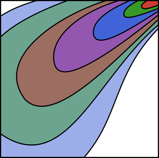
Elliptical family

Definition

The easiest families of copulas are the one derived from known families of random vectors, and the first presented one are, generally, the Elliptical families (in particular, the Gaussian and Student families are very standard in the litterature).

Definition: Spherical and elliptical random vectors

A random vector $\mathit{X}$ is said to be spherical if for all orthogonal matrix $\mathit{A}\in O_d(\mathbb{R})$, $\mathit{A}\mathit{X}\sim \mathit{X}$.

For every matrix $\mathit{B}$ and vector $\mathit{c}$, the random vector $\mathit{B}\mathit{X}+\mathit{c}$ is then said to be elliptical.

Spherical random vectors have several interesting properties. First, the shape of the distribution must be the same in every direction since it is stable by rotations. Moreover, their characteristic functions (c.f.) only depend on the norm of their arguments. Indeed, for any $\mathit{A}\in O_d(\mathbb{R})$,

$$\varphi (\mathit{t})=\mathbb{E}\left(e^{⟨\mathit{t},\mathit{X}⟩}\right)=\mathbb{E}\left(e^{⟨\mathit{t},\mathit{A}\mathit{X}⟩}\right)=\mathbb{E}\left(e^{⟨\mathit{A}\mathit{t},\mathit{X}⟩}\right)=\varphi (\mathit{A}\mathit{t}).$$

We can therefore express this characteristic function as $\varphi (\mathit{t})=\psi (\Vert \mathit{t}{\Vert }_2^2)$, where $\psi$ is a function that characterizes the spherical family, called the generator of the family. Any characteristic function that can be expressed as a function of the norm of its argument is the characteristic function of a spherical random vector, since $\Vert \mathit{A}\mathit{t}{\Vert }_2=\Vert \mathit{t}{\Vert }_2$ for any orthogonal matrix $\mathit{A}$.

This class contains the (multivariate) Normal and Student distributions, and it is easy to construct others if needed. This is a generalization of the family of Gaussian random vectors, and they benefit from several nice properties of the former, among which, particularly interesting, the stability by convolution. Indeed, convolutions correspond to product of characteristic functions, and

$$\varphi (\mathit{t})=\prod _{i=1}^n{\varphi }_i(\mathit{t})=\prod _{i=1}^n{\psi }_i(\Vert \mathit{t}{\Vert }_2^2)=\psi (\Vert \mathit{t}{\Vert }_2^2),$$

which is still a function of only the norm of $\mathit{t}$.

To fix ideas, for Gaussian random vectors, $\psi (t)=e^{-\frac{t^2}{2}}$.

Sampling with Distributions.jl

Elliptical random vectors in the Gaussian and Student families are available from Distributions.jl:

using Distributions
Σ = [1 0.5
    0.5 1] # variance-covariance matrix.
ν = 3 # number of degrees of freedom for the student.
N = MvNormal(Σ)

ZeroMeanFullNormal(
dim: 2
μ: Zeros(2)
Σ: [1.0 0.5; 0.5 1.0]
)

T = MvTDist(ν,Σ)

Distributions.GenericMvTDist{Float64, PDMats.PDMat{Float64, Matrix{Float64}, LinearAlgebra.Cholesky{Float64, Matrix{Float64}}}, FillArrays.Zeros{Float64, 1, Tuple{Base.OneTo{Int64}}}}(
df: 3.0
dim: 2
μ: Zeros(2)
Σ: [1.0 0.5; 0.5 1.0]
)

Elliptical copulas are simply copulas of elliptical distributions. This simplicity of definition is paid for in the expression of the copulas itself: the obtained function has usually no better expression than:

$$C=F\circ (F_1^{-1},...,F_d^{-1}),$$

where $F_i^{-1}$ denotes the almost-inverse of $F_i$, that is:

$$\mathrm{\forall }u\in [0,1],F_i^{-1}(u)=inf\{x:F_i(x)\ge u\},$$

and $F_i$ is usually hard to express from the elliptical assumptions.

Moreover, the form of dependence structures that can be reached inside this class is restricted. The elliptical copulas are parametrized by the corresponding univariate spherical generator and a correlation matrix, which is a very simple structure. See also [23–25] for details on these copulas.

On the other hand, there exist performant estimators of high-dimensional covariance matrices, and a large theory is built on the elliptical assumption of high dimensional random vectors, see e.g., [26–28] among others. See also [29] for a recent work on nonparametric estimation of the underlying univariate spherical distribution.

Note on internal implementation

If the exposition we just did on characteristic functions of Elliptical random vectors is fundamental to the definition of elliptical copulas, the package does not use this at all to function, and rather rely on the existence of multivariate and corresponding univariate families of distributions in Distributions.jl.

You can obtain these elliptical copulas by the following code:

using Copulas
Σ = [1 0.5
     0.5 1] # variance-covariance matrix.
ν = 3 # number of degrees of freedom for the student.
C_N = GaussianCopula(Σ)
C_T = TCopula(ν,Σ)

Examples

To construct, e.g., a Student copula, you need to provide the Correlation matrix and the number of degree of freedom, as follows:

using Copulas, Distributions
Σ = [1 0.5
    0.5 1] # variance-covariance matrix.
ν = 3 # number of degrees of freedom
C = TCopula(ν,Σ)

TCopula{2, Int64, Matrix{Float64}}(Σ = [1.0 0.5; 0.5 1.0]))

You can sample it and compute its density and distribution functions via the standard interface. We could try to fit a GaussianCopula on the sampled data, even if we already know that the tails will not be properly taken into account:

u = rand(C,1000)
Ĉ = fit(GaussianCopula,u) # to fit on the sampled data.

GaussianCopula{2, Matrix{Float64}}(Σ = [1.0 0.5069034434223326; 0.5069034434223326 1.0]))

We see that the estimation we have on the correlation matrix is quite good, but rest assured that the tails of the distributions are not the same at all. To see that, let's plot the lower tail function (see [3]) for both copulas:

using Plots
chi(C,u) = 2 * log(1-u) / log(1 - 2u + cdf(C,[u,u])) -1
u = 0.5:0.03:0.99
plot(u,  chi.(Ref(C),u), label="True student copula")
plot!(u, chi.(Ref(Ĉ),u), label="Estimated Gaussian copula")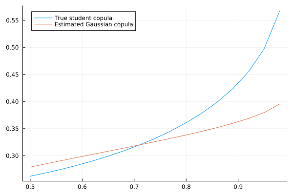

Visual: Gaussian vs Student (same correlation)

using Plots
Σ = [1 0.7; 0.7 1]
ν = 4
CG = GaussianCopula(Σ)
CT = TCopula(ν, Σ)
plot(plot(CG), plot(CT); layout=(1,2))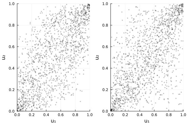

Conditional on original scale via SklarDist

XG = SklarDist(CG, (Normal(), Normal()))
XT = SklarDist(CT, (Normal(), Normal()))
X1G = condition(XG, 2, 0.0)
X1T = condition(XT, 2, 0.0)
xgrid = range(quantile(X1T, 0.001), quantile(X1T, 0.999); length=401)
plot(xgrid, Distributions.cdf.(Ref(X1G), xgrid); label="Gaussian", xlabel="x", ylabel="cdf",
    title="F_{X1|X2=0}")
plot!(xgrid, Distributions.cdf.(Ref(X1T), xgrid); label="Student")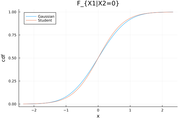

The difference between the two is not very strong.

Conditionals and distortions

For an elliptical copula built from an underlying elliptical vector $X=(X_1,\dots ,X_d)$ with correlation matrix $\mathrm{\Sigma }$ and univariate CDFs $(F_i)$, conditioning follows the standard elliptical identities. Partition indices as $I\cup J=\{1,\dots ,d\}$ and conformably partition $\mathrm{\Sigma }$ as

$$\mathrm{\Sigma }=\left(\begin{array}{cc}{\mathrm{\Sigma }}_{II}& {\mathrm{\Sigma }}_{IJ}\\ {\mathrm{\Sigma }}_{JI}& {\mathrm{\Sigma }}_{JJ}\end{array}\right).$$

• For the Gaussian copula, the conditional law $X_I|X_J=x_J$ is Gaussian with ${\mu }_{I|J}={\mathrm{\Sigma }}_{IJ}{\mathrm{\Sigma }}_{JJ}^{-1}{x}_J,{\mathrm{\Sigma }}_{I|J}={\mathrm{\Sigma }}_{II}-{\mathrm{\Sigma }}_{IJ}{\mathrm{\Sigma }}_{JJ}^{-1}{\mathrm{\Sigma }}_{JI}.$ Mapping to the copula scale with $u_k=\mathrm{\Phi }(x_k)$ and $x_k={\mathrm{\Phi }}^{-1}(u_k)$ yields the conditional copula via $C_{I|J}({\mathit{u}}_I\mid {\mathit{u}}_J)=Pr[X_I\le {\mathrm{\Phi }}^{-1}({\mathit{u}}_I)|X_J={\mathrm{\Phi }}^{-1}({\mathit{u}}_J)],$ and the univariate conditional distortions $H_{i|J}(u\mid {\mathit{u}}_J)=Pr[X_i\le {\mathrm{\Phi }}^{-1}(u)|X_J={\mathrm{\Phi }}^{-1}({\mathit{u}}_J)]=\mathrm{\Phi }(\frac{{\mathrm{\Phi }}^{-1}(u)-{\mu }_{i|J}}{\sqrt{{\mathrm{\Sigma }}_{i|J}}}).$

• For the Student-$t$ copula with degrees of freedom $\nu$, one uses the standard conditional-$t$ result: $X_I|X_J=x_J\sim t_p({\mu }_{I|J},\frac{\nu +q_J}{\nu +r_J}{\mathrm{\Sigma }}_{I|J},\nu +|J|)$, where $q_J=|J|$ and $r_J=(x_J{)}^{\mathrm{\top }}{\mathrm{\Sigma }}_{JJ}^{-1}{x}_J$.

    With $u_k = F_t(x_k;\,\nu)$ and $x_k = F_t^{-1}(u_k;\,\nu)$ (standard univariate $t$ with df $\nu$), this provides closed forms for $C_{I|J}$ and for
  
    $$H_{i|J}(u\mid\boldsymbol u_J) = F_t\!\Big(\,F_t^{-1}(u;\,\nu)\,;\,\mu_{i|J},\,\tfrac{\nu + r_J}{\nu + q_J}\,\Sigma_{i|J},\,\nu+|J|\Big),$$
  
    where $q_J=|J|$, $r_J= x_J^\top\Sigma_{JJ}^{-1}x_J$, and $F_t(\cdot;\,\mu,\sigma^2,\nu)$ is the univariate non-standard $t$ CDF.

These formulas are what the implementation relies on (via SklarDist for original scale and via marginal CDF transforms for the copula scale) to compute condition and the associated distortions efficiently.

Copulas.EllipticalCopula Type

EllipticalCopula{d,MT}

This is an abstract type. It implements an interface for all Elliptical copulas. We construct internally elliptical copulas using the sklar's theorem, by considering the copula $C$ to be defined as :

$$C=F\circ (F_1^{-1},...,F_d^{-1}),$$

where $F$ and $F_1,...,F_d$ are respectively the multivariate distribution function of some elliptical random vector and the univariate distribution function of its marginals. For a type MyCop <: EllipitcalCopula, it is necessary to implement the following methods:

• N(::Type{MyCOp}), returning the constructor of the elliptical random vector from its correlation matrix. For example, N(GaussianCopula) simply returns MvNormal from Distributions.jl.

• U(::Type{MyCOp}), returning the constructor for the univariate marginal, usually in standardized form. For example, U(GaussianCopula) returns Normal from Distributions.jl.

From these two functions, the abstract type provides a fully functional copula.

Details

Recall the definition of spherical random vectors:

Definition - Spherical and elliptical random vectors

A random vector $\mathit{X}$ is said to be spherical if for all orthogonal matrix $\mathit{A}\in O_d(\mathbb{R})$, $\mathit{A}\mathit{X}\sim \mathit{X}$.

For every matrix $\mathit{B}$ and vector $\mathit{c}$, the random vector $\mathit{B}\mathit{X}+\mathit{c}$ is then said to be elliptical.

Recall that spherical random vectors are random vectors which characteristic functions (c.f.) only depend on the norm of their arguments. Indeed, for any $\mathit{A}\in O_d(\mathbb{R})$,

$$\varphi (\mathit{t})=\mathbb{E}\left(e^{⟨\mathit{t},\mathit{X}⟩}\right)=\mathbb{E}\left(e^{⟨\mathit{t},\mathit{A}\mathit{X}⟩}\right)=\mathbb{E}\left(e^{⟨\mathit{A}\mathit{t},\mathit{X}⟩}\right)=\varphi (\mathit{A}\mathit{t}).$$

We can therefore express this characteristic function as $\varphi (\mathit{t})=\psi (\Vert \mathit{t}{\Vert }_2^2)$, where $\psi$ is a function that characterizes the spherical family, called the generator of the family. Any characteristic function that can be expressed as a function of the norm of its argument is the characteristic function of a spherical random vector, since $\Vert \mathit{A}\mathit{t}{\Vert }_2=\Vert \mathit{t}{\Vert }_2$ for any orthogonal matrix $\mathit{A}$.

However, note that this is not how the underlying code is working, we do not check for validity of the proposed generator (we dont even use it). You can construct such an elliptical family using simply Sklar:

struct MyElliptical{d,T} <: EllipticalCopula{d,T}
    θ:T
end
U(::Type{MyElliptical{d,T}}) where {d,T} # Distribution of the univaraite marginals, Normal() for the Gaussian case. 
N(::Type{MyElliptical{d,T}}) where {d,T} # Distribution of the mutlivariate random vector, MvNormal(C.Σ) for the Gaussian case.

These two functions are enough to implement the rest of the interface.

References:

• [3] Nelsen, Roger B. An introduction to copulas. Springer, 2006.

source

Available models

GaussianCopula

Copulas.GaussianCopula Type

GaussianCopula{d, MT}

Fields:

• Σ::MT — correlation matrix (the constructor coerces the input to a correlation matrix).

Constructors

GaussianCopula(Σ)
GaussianCopula(d, ρ)
GaussianCopula{d}(Σ)
GaussianCopula{d}(ρ)

Where Σ is a (symmetric) covariance or correlation matrix. The two-argument form with (d, ρ) builds the equicorrelation matrix with ones on the diagonal and constant off-diagonal correlation ρ:

Σ = fill(ρ, d, d); Σ[diagind(Σ)] .= 1
C = GaussianCopula(d, ρ)            # == GaussianCopula(Σ)

Validity domain (equicorrelated PD matrix): -1/(d-1) < ρ < 1. The boundary ρ = -1/(d-1) is singular and rejected. If ρ == 0, the resulting GaussianCopula represents independence, as it does for any diagonal matrix.

The Gaussian copula is the copula of a multivariate normal distribution. It is defined by

$$C(\mathbf{x};\mathbf{\Sigma })=F_{\mathrm{\Sigma }}(F_{\mathrm{\Sigma },1}^{-1}(x_1),\dots ,F_{\mathrm{\Sigma },d}^{-1}(x_d)),$$

where $F_{\mathrm{\Sigma }}$ is the cdf of a centered multivariate normal with covariance/correlation $\mathrm{\Sigma }$ and $F_{\mathrm{\Sigma },i}$ its i-th marginal cdf.

Example usage:

C = GaussianCopula(Σ)
u = rand(C, 1000)
pdf(C, u); cdf(C, u)
Ĉ = fit(GaussianCopula, u)

Special case:

• If isdiag(Σ), the GaussianCopula represents independence while retaining its concrete family type.

References:

• [3] Nelsen, Roger B. An introduction to copulas. Springer, 2006.

source

Targeting a Pearson correlation: the Nataf correction

The parameter matrix of a GaussianCopula is the correlation matrix of the underlying Gaussian random vector. When the copula is coupled to non-Gaussian marginals through SklarDist, that parameter is not the Pearson correlation of the resulting random vector, because Pearson correlation depends on the marginals (only rank-based measures such as Kendall's τ or Spearman's ρ are marginal-free, see the dependence measures page):

using Copulas, Distributions, Statistics, Random
rng = Xoshiro(1)
C = GaussianCopula([1.0 0.7; 0.7 1.0])
D = SklarDist(C, (LogNormal(0, 0.8), LogNormal(0, 0.8)))
cor(rand(rng, D, 10^5)') # although the copula parameter is 0.7...

2×2 Matrix{Float64}:
 1.0       0.631666
 0.631666  1.0

The Nataf correction [20, 21] inverts this distortion: it computes the copula parameter matrix that makes the SklarDist attain a target Pearson correlation matrix for the given marginals:

m  = (LogNormal(0, 0.8), LogNormal(0, 0.8))
R₀ = Nataf(m, [1.0 0.7; 0.7 1.0])

2×2 Matrix{Float64}:
 1.0       0.761043
 0.761043  1.0

D = SklarDist(GaussianCopula(R₀), m)
cor(rand(rng, D, 10^5)') # ≈ 0.7 as requested.

2×2 Matrix{Float64}:
 1.0       0.702896
 0.702896  1.0

Since non-Gaussian marginals cannot attain every Pearson correlation (the Fréchet-Hoeffding bounds of the pair), an unattainable target throws an error reporting the attainable range. Pairs among Normal, LogNormal, and Uniform margins use closed-form corrections; other marginals go through a Gauss-Hermite quadrature.

Copulas.Nataf Function

Nataf(margins, R; nodes=32)
Nataf(margins, ρ::Real; nodes=32)

Nataf correction [20, 21]: compute the correlation matrix for a GaussianCopula such that the SklarDist built from it and the given margins has Pearson correlation matrix R.

A Gaussian copula with parameter ${\rho }_0$ induces, once the margins are applied, a Pearson correlation that depends on the shape of the margins and equals ${\rho }_0$ only when the margins are themselves Gaussian. Matching a Pearson target $\rho$ therefore means inverting, for each pair of margins,

$$\rho ({\rho }_0)=\mathbb{E}[g_i(Z_i)g_j(Z_j)],(Z_i,Z_j)\sim \mathcal{N}(0,\left(\begin{array}{cc}1& {\rho }_0\\ {\rho }_0& 1\end{array}\right)),$$

where $g_k(z)=(F_k^{-1}(\mathrm{\Phi }(z))-{\mu }_k)/{\sigma }_k$ is the standardized margin pulled back to standard normal space. The expectation is evaluated with a product Gauss-Hermite rule and, since it is increasing in ${\rho }_0$, inverted by a bracketed root search.

Arguments

• margins: a Tuple or vector of univariate distributions, each with finite mean and finite positive standard deviation.

• R: the target Pearson correlation matrix (or a single target correlation ρ when there are exactly two margins, in which case the corrected scalar is returned).

• nodes: number of Gauss-Hermite nodes per dimension. The default is accurate to about 1e-8 for well-behaved margins; heavy-tailed or strongly skewed margins converge more slowly and want more nodes.

Zero targets map to exactly zero. Pairs whose induced correlation is known analytically skip the quadrature and use the closed form instead: Normal-Normal pairs (the identity, so Gaussian margins reproduce R exactly), LogNormal-LogNormal pairs (${\rho }_0=\log (1+\rho \sqrt{(e^{s_i^2}-1)(e^{s_j^2}-1)})/(s_i{s}_j)$), and all pairs among Normal, LogNormal, and Uniform margins. Because non-Gaussian margins cannot attain every Pearson correlation (the Fréchet-Hoeffding bounds), a target outside the attainable range throws an error naming the pair and the range. Targets on the attainable boundary snap just inside $\pm 1$, so the result stays usable by the GaussianCopula constructor; the corrected matrix is nevertheless not guaranteed to stay positive definite for extreme targets in dimension $d>2$, and the GaussianCopula constructor validates it.

The computation is type-generic and follows the precision of the inputs: BigFloat targets or margin parameters yield BigFloat results, at full precision on the closed-form paths. Two caveats on the generic quadrature path: its nodes are computed in Float64, and it requires margins whose quantile accepts the working type — some quantiles in Distributions.jl (e.g. Gamma, Beta) are implemented for machine floats only and throw a MethodError for BigFloat arguments.

Example

using Copulas, Distributions, Statistics

m  = (LogNormal(0, 0.8), Gamma(1, 2), Beta(1, 2))
R0 = [1 0.7 0.3; 0.7 1 0.5; 0.3 0.5 1]

D = SklarDist(GaussianCopula(Nataf(m, R0)), m)
cor(rand(D, 10^6)') # ≈ R0, while GaussianCopula(R0) directly would miss the target.

References:

• [20] Nataf, A. (1962). Détermination des distributions de probabilités dont les marges sont données.

• [21] Liu, P.-L., & Der Kiureghian, A. (1986). Multivariate distribution models with prescribed marginals and covariances.

source

TCopula

Copulas.TCopula Type

TCopula{d, Tν, MT}

Fields:

• df::Tν — degrees of freedom

• Σ::MT — correlation matrix

Constructor

TCopula(df, Σ)
TCopula{d}(df, Σ)

The Student t copula is the copula of a multivariate Student t distribution. It is defined by

$$C(\mathbf{x};\nu ,\mathbf{\Sigma })=F_{\nu ,\mathrm{\Sigma }}(F_{\nu ,\mathrm{\Sigma },1}^{-1}(x_1),\dots ,F_{\nu ,\mathrm{\Sigma },d}^{-1}(x_d)),$$

where $F_{\nu ,\mathrm{\Sigma }}$ is the cdf of a centered multivariate t with correlation $\mathrm{\Sigma }$ and $\nu$ degrees of freedom.

Example usage:

C = TCopula(2, Σ)
u = rand(C, 1000)
pdf(C, u); cdf(C, u)
Ĉ = fit(TCopula, u)

References:

• [3] Nelsen, Roger B. An introduction to copulas. Springer, 2006.

source

References

2. R. B. Nelsen. An Introduction to Copulas. 2nd ed Edition, Springer Series in Statistics (Springer, New York, 2006).

3. A. Nataf. Détermination des distributions de probabilités dont les marges sont données. Comptes Rendus de l'Académie des Sciences 255, 42–43 (1962).

4. P.-L. Liu and A. Der Kiureghian. Multivariate distribution models with prescribed marginals and covariances. Probabilistic Engineering Mechanics 1, 105–112 (1986).

5. G. Frahm, M. Junker and A. Szimayer. Elliptical Copulas: Applicability and Limitations. Statistics & Probability Letters 63, 275–286 (2003).

6. E. Gómez, M. A. Gómez-villegas and J. M. Marín. A Survey on Continuous Elliptical Vector Distributions. Revista Matemática Complutense 16, 345–361 (2003).

7. M.-P. Côté and C. Genest. Dependence in a Background Risk Model. Journal of Multivariate Analysis 172, 28–46 (2019).

8. G. Elidan. Copulas in Machine Learning. In: Copulae in Mathematical and Quantitative Finance, Vol. 213, edited by P. Jaworski, F. Durante and W. K. Härdle (Springer Berlin Heidelberg, Berlin, Heidelberg, 2013); pp. 39–60.

9. J. Friedman, T. Hastie and R. Tibshirani. Applications of the Lasso and Grouped Lasso to the Estimation of Sparse Graphical Models (Technical report, Stanford University, 2010).

10. D. Müller and C. Czado. Dependence Modelling in Ultra High Dimensions with Vine Copulas and the Graphical Lasso. Computational Statistics & Data Analysis 137, 211–232 (2019).

11. A. Derumigny and J.-D. Fermanian. Identifiability and Estimation of Meta-Elliptical Copula Generators. Journal of Multivariate Analysis, 104962 (2022).