Fitting interface

This section summarizes how to fit copulas (and Sklar distributions) in Copulas.jl, without going into family-specific details.

---

Data conventions

• We work with pseudo-observations U ∈ (0,1)^{d×n} (rows = dimensions, columns = observations). Use pseudos(X) to obtain normalized ranks from raw data X.

• Rank-based routines (tau / rho / beta / gamma) assume pseudo-observations.

• StatsBase pairwise correlation helpers use the n×d convention; internally we transpose as needed (e.g., U').

---

Main calls

Copula only (object)

using Copulas, Random, StatsBase, Distributions, Plots
Ctrue = GumbelCopula(2, 3.0)
U = rand(Ctrue, 2_000)
Ĉ = fit(GumbelCopula, U; method=:mle)
Ĉ

GumbelCopula{2, Float64}(θ = 3.101831168554804,)

Returns only the fitted copula Ĉ::CT (high-level shortcut).

Full model (with metadata)

M = fit(CopulaModel, GumbelCopula, U; method=:default)
M

────────────────────────────────────────────────────────────────────────────────
[ CopulaModel: Archimedean d=2 ]
────────────────────────────────────────────────────────────────────────────────
Method:                mle
Number of observations: 2000
────────────────────────────────────────────────────────────────────────────────
[ Fit metrics ]
────────────────────────────────────────────────────────────────────────────────
Null Loglikelihood:          0.0000
Loglikelihood:            1496.9015
LR (vs indep.):        2993.80 ~ χ²(1)  ⇒  p = <1e-16
AIC:                   -2991.803
BIC:                   -2986.202
Converged:             true
Iterations:            4
Elapsed:               0.007s
────────────────────────────────────────────────────────────────────────────────
[ Dependence metrics ]
────────────────────────────────────────────────────────────────────────────────
Kendall τ:             0.6776
Spearman ρ:            0.8580
Blomqvist β:           0.6813
Gini γ:                0.7351
Upper λᵤ:              0.7496
Lower λₗ:              0.0021
Entropy ι:             -0.7644
────────────────────────────────────────────────────────────────────────────────
[ Copula parameters ] (vcov=hessian)
────────────────────────────────────────────────────────────────────────────────
Parameter    Estimate   Std.Err   z-value    p-val     95% Lo     95% Hi
θ              3.1018    0.0576    53.892   <1e-16     2.9890     3.2146

Returns a CopulaModel with:

• result (the fitted copula), n, ll (log-likelihood),

• method, converged, iterations, elapsed_sec,

• vcov (if available),

• method_details (a NamedTuple with method-specific metadata).

---

Behavior & conventions (important)

• $fit$ operates on types, not on pre-constructed instances. Pass a copula or Sklar type, e.g. fit(GumbelCopula, U) or fit(CopulaModel, SklarDist{ClaytonCopula,Tuple{Normal,LogNormal}}, X). If you already have an instance C0, re-estimate its parameters with fit(typeof(C0), U).

• Default method selection. Each family exposes allowed fitting strategies via _available_fitting_methods(CT, d). With method = :default, the first element of that tuple is used. Example: Copulas._available_fitting_methods(MyCopula, d).

• CopulaModel is the full result returned by Distributions.fit(::Type{CopulaModel}, ...). The lightweight shortcut fit(MyCopula, U) returns only a copula; use fit(CopulaModel, ...) to get diagnostics and metadata.

---

CopulaModel interface (summary)

The CopulaModel{CT} <: StatsBase.StatisticalModel supports the standard StatsBase API and a few additional fields:

Function / Field	Description
Field M.ll	Log-likelihood at the optimum (numeric field stored in the model).
nobs(M)	Number of observations used in the fit.
deviance(M)	Deviance (= −2 · M.ll).
nullloglikelihood(M)	Log-likelihood under independence with same margins (available for Sklar fits).
nulldeviance(M)	Deviance of the null model (−2 · nullloglikelihood(M)).
aic(M) / bic(M)	Information criteria from $StatsBase.jl$
aicc(M) / hqc(M)	Information criteria from $Copulas.jl$
coef(M) / coefnames(M)	Estimated parameters and their names.
vcov(M)	Parameter variance–covariance matrix (may be nothing).
stderror(M) / confint(M; level=0.95)	Standard errors and Wald confidence intervals (require vcov(M) ≠ nothing).
residuals(M; transform=:uniform | :normal)	Rosenblatt residuals on [0,1] or Normal scale (requires method_details[:U]).
predict(M; what=:cdf|:pdf|:simulate, ...)	CDF/PDF at newdata, or simulation (nsim; default nsim = M.n if nsim == 0).

Examples

# Information criteria
StatsBase.aic(M)
StatsBase.bic(M)
Copulas.aicc(M)
Copulas.hqc(M)

-2989.7465401775858

# Standard errors and Wald CIs
StatsBase.stderror(M)
StatsBase.confint(M; level=0.95)

([2.9890222519185112], [3.214640085191097])

# Rosenblatt residuals
R  = StatsBase.residuals(M; transform=:uniform)
RN = StatsBase.residuals(M; transform=:normal)
(size(R), size(RN))

((2, 2000), (2, 2000))

# Predictions and simulation
P  = StatsBase.predict(M; what=:cdf, newdata=rand(2, 5))   # CDF at 5 points
F  = StatsBase.predict(M; what=:pdf, newdata=rand(2, 5))   # PDF at 5 points
X̂  = StatsBase.predict(M; what=:simulate, nsim=1_000)     # simulate 1,000 obs
(size(P), size(F), size(X̂))

((5,), (5,), (2, 1000))

---

Covariance estimation (vcov) and inference

When fitting with fit(CopulaModel, ...), the keyword vcov=true triggers estimation of the parameter covariance matrix.

Default. vcov = true. Covariance is computed automatically unless the user disables it (vcov=false) or a family turns it off internally (e.g., TCopula, FGMCopula, tEVCopula) when required derivatives are not implemented.

The internal dispatcher _vcov(CT, U, θ̂; method, override) selects the estimator:

Symbol	Description
:hessian	Inverse observed information (−Hessian of the log-likelihood). Default for method = :mle.
:godambe	Godambe (sandwich) estimator based on score-type functions. Used for rank-based fits.
:godambe_pairwise	Pairwise Godambe using all variable pairs.
:jackknife	Leave-one-out jackknife approximation (robust fallback).
:bootstrap	Bootstrap approximation (√n resamples, up to 200).

You can override the choice via vcov_method:

M2 = fit(CopulaModel, GumbelCopula, U; method=:mle, vcov=true, vcov_method=:bootstrap, derived_measures=false)
StatsBase.vcov(M2) isa AbstractMatrix

true

Each method returns a symmetric (positive semi-definite) matrix Vθ, stored as M.vcov and exposed by StatsBase.vcov(M).

Fallbacks. If non-finite values appear in Hessian/Godambe computations, the algorithm automatically falls back (first to :bootstrap; if instability persists, to :jackknife).

Note. In the example above we set derived_measures=false, which disables the automatic calculation and storage of dependence measures (e.g., Kendall’s τ, Spearman’s ρ, Blomqvist’s β, , Gini's γ, upper/lower tail coefficients, entropy). By default this is enabled. Disabling it reduces computation and memory footprint and omits the Dependence metrics section in the REPL summary.

Joint margins + copula (Sklar)

You can pass the sklar_method parameter as:

• :ifm: fits parametric margins and maps data to pseudo-scale via their CDFs.

• :ecdf: uses empirical pseudo-observations (ranks).

Notes

• Use sklar_method = :ifm when margins are plausibly parametric and you want a model-based projection; use :ecdf to avoid margin misspecification.

• margins_kwargs is a single NamedTuple applied to every marginal fit. For heterogeneous options, fit margins manually and then fit the copula on the resulting pseudo-data.

• The model’s null_ll (for LR tests) is the log-likelihood under independence with the same margins.

S = SklarDist(ClaytonCopula(2, 5), (Normal(), LogNormal(0, 0.5)))
X = rand(S, 1000)
Ŝ = fit(CopulaModel, SklarDist{ClaytonCopula,Tuple{Normal,LogNormal}}, X;
	sklar_method=:ifm, # or :ecdf
	copula_method=:default, # see next section.
	margins_kwargs=NamedTuple(), copula_kwargs=NamedTuple()) # options will be passed down to fitting functions.
Ŝ

────────────────────────────────────────────────────────────────────────────────
[ CopulaModel: SklarDist ] (Copula=Archimedean d=2, Margins=(Normal, LogNormal))
────────────────────────────────────────────────────────────────────────────────
Copula:                Archimedean d=2
Margins:               (Normal, LogNormal)
Methods:               copula=mle, sklar=ifm
Number of observations: 1000
────────────────────────────────────────────────────────────────────────────────
[ Fit metrics ]
────────────────────────────────────────────────────────────────────────────────
Null Loglikelihood:      -2166.1883
Loglikelihood:           -1188.6310
LR (vs indep.):        1955.11 ~ χ²(1)  ⇒  p = <1e-16
AIC:                   2379.262
BIC:                   2384.170
Converged:             true
Iterations:            3
Elapsed:               0.006s
────────────────────────────────────────────────────────────────────────────────
[ Dependence metrics ]
────────────────────────────────────────────────────────────────────────────────
Kendall τ:             0.7189
Spearman ρ:            0.8880
Blomqvist β:           0.7515
Gini γ:                0.7727
Upper λᵤ:              0.0000
Lower λₗ:              0.8732
Entropy ι:             -0.9889
────────────────────────────────────────────────────────────────────────────────
[ Copula parameters ] (vcov=hessian)
────────────────────────────────────────────────────────────────────────────────
Parameter    Estimate   Std.Err   z-value    p-val     95% Lo     95% Hi
θ              5.1139    0.1688    30.301   <1e-16     4.7831     5.4447
────────────────────────────────────────────────────────────────────────────────
[ Marginals ]
────────────────────────────────────────────────────────────────────────────────
Margin Dist       Param    Estimate   Std.Err 95% CI
#1     Normal     μ          0.0275    0.0318 [-0.0348, 0.0899]
                  σ          1.0063    0.0225 [0.9622, 1.0504]
#2     LogNormal  μ          0.0063    0.0160 [-0.0250, 0.0376]
                  σ          0.5047    0.0113 [0.4826, 0.5268]

plot(Ŝ.result)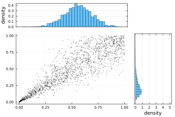

---

Available fitting methods

The names and availability of fitting methods depend on the family. Inspect them via:

Copulas._available_fitting_methods(ClaytonCopula, 3)

(:mle, :itau, :irho, :ibeta)

The first method in the list is used by default.

Short descriptions

• :mle — Maximum likelihood over U. Recommended when a stable density and a good reparameterization exist.

• :itau — Kendall inverse: matches theoretical tau(C) to empirical tau(U). Ideal for single-parameter families with a monotone inverse.

• :irho — Spearman inverse: analogous to rho; can use scalar or matrix objectives (e.g., multivariate Gaussians).

• :ibeta — Blomqvist inverse: scalar; only valid for families with ≤ 1 free parameter.

Remark. Rank-based methods require that the number of free parameters does not exceed the information contained in the chosen coefficient(s); :ibeta enforces this explicitly.

For extreme-value copulas, :mle / :iupper may rely on the Pickands function A(t) and its derivatives (A, dA, d²A) with Brent-type inversion.

Nonparametric fits (Empirical Copulas)

In addition to parametric families (MLE / rank-based), Copulas.jl exposes several nonparametric or empirical constructions that can be fit through the same high-level API:

• EmpiricalCopula (Deheuvels)

• BetaCopula

• BernsteinCopula

• CheckerboardCopula

• EmpiricalEVCopula (built from EmpiricalEVTail, bivariate extreme-value case)

See the dedicated page for theory, properties, and references: Empirical models.

All StatsBase / StatsModels functionality works identically for these copulas: you can call coef, aic, bic, deviance, predict, residuals, etc., and obtain a full CopulaModel object with the same structure and printing behavior.

The only difference is that empirical models are parameter-free (dof(M) = 0), so vcov(M), stderror(M), and confint(M) return nothing, and information criteria reduce to AIC = BIC = −2 · loglikelihood. Otherwise, all features—including the computation of dependence measures and the REPL summary—behave exactly the same.