<!– This file is generated from README.md by docs/sync_homepage.jl. –>

Welcome to Copulas.jl! ​

The Copulas.jl package provides a large collection of models for dependence structures of real random vectors, known as copulas, with a wide selection of features:

• random number generation

• evaluation of (log)density and distribution functions

• copula-based multivariate distributions via Sklar's theorem

• fitting procedures, model diagnostics, and automatic family selection

• dependence metrics and tail coefficients

• marginalization, conditioning, and Rosenblatt transforms

• resampling-based hypothesis tests for dependence assumptions and goodness of fit

Since copulas are distribution functions, we integrate with the Distributions.jl API. This integration supports interoperability with other packages based on that API, such as Turing.jl. The precise 1.0 guarantees, including the treatment of singular and mixed measures, are defined on the Public API page.

Usually, users who work with copulas turn to the R package copula. While still well-maintained and regularly updated, the R package copula is a complicated code base in terms of readability, extensibility, reliability, and maintenance. This package aims to provide a lightweight, fast, reliable, and maintainable copula implementation in native Julia. Core numerical paths are written generically where practical and model representations preserve their documented numeric types. Individual algorithms and external numerical backends may have narrower support; unsupported precision should fail explicitly rather than be silently narrowed. GPU and arbitrary-precision support are therefore operation- and backend-dependent rather than package-wide guarantees. See the Public API page for the normative numeric contract.

The package revolves around two main types:

• Copula, the abstract supertype of all copulas

• SklarDist, the type for multivariate compound distributions via Sklar's theorem

Getting started ​

The package is registered in Julia's General registry so you may simply install the package by running :

] add Copulas

The API contains random number generation, cdf and pdf evaluation, and the fit function from Distributions.jl. A typical use case might look like this:

using Copulas, Distributions, Random, Plots
X₁ = Gamma(2,3)
X₂ = Beta(1,4)
X₃ = Normal()
C = ClaytonCopula(3,5.2) # A 3-variate Clayton copula with θ = 5.2
D = SklarDist(C,(X₁,X₂,X₃)) # The final distribution

simu = rand(D,1000) # Generate a dataset
D̂ = fit(SklarDist{ClaytonCopula,Tuple{Gamma,Beta,Normal}}, simu) # estimate a model
plot(D̂) # plot the result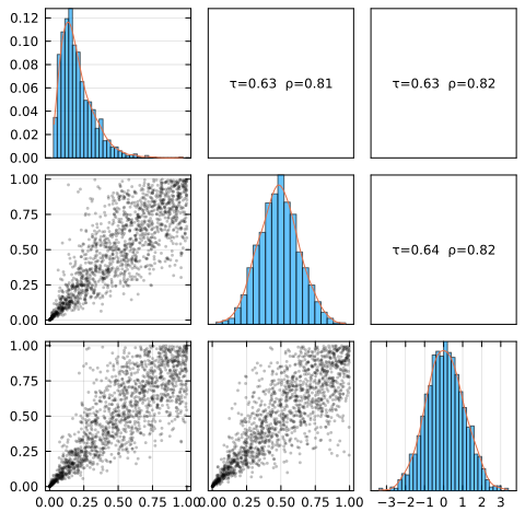

The list of available copula models is very large; browse the Bestiary for definitions, parameterizations, constructors, and model-specific caveats. The general implementation philosophy is for the code to follow the mathematical boundaries of the implemented concepts. For example, this is the only implementation we know (in any language) that allows for all Archimedean copulas to be sampled: we use the Williamson transformation for non-standard generators, including user-provided black-box ones.

Feature comparison ​

Other Julia packages cover related use cases. BivariateCopulas.jl focuses on a compact set of bivariate copulas, joint distributions, conditioning, and visualization. DatagenCopulaBased.jl focuses on data generation, including selected nested and chained constructions. The comparison below summarizes capabilities documented by each project; “Not documented” means that the linked public README does not advertise the feature, not that no implementation can exist.

The table compares public scope rather than runtime performance; algorithmic cost depends strongly on the family, dimension, and requested operation.

Quick API Tour ​

Here is a practical tour of the main public workflows. For precise behavioral guarantees see the Public API; for theory and model-specific guidance see the Manual and Bestiary.

Copulas and Sklar distributions ​

You can construct a copula object with their respective constructors. They behave like multivariate distributions from Distributions.jl and respect their API:

using Copulas, Distributions, Random, StatsBase
# A 3-variate Clayton copula
C = ClaytonCopula(3, 2.0)
U = rand(C, 5)
Distributions.loglikelihood(C, U)

7.7827056787289335

To build multivariate distributions, you can compose a copula with marginals via Sklar’s theorem:

X₁, X₂, X₃ = Gamma(2,3), Beta(1,5), LogNormal(0,1)
C2 = GumbelCopula(3, 1.7)
D  = SklarDist(C2, (X₁, X₂, X₃))
rand(D, 3)
pdf(D, rand(3))

0.0007812359657052404

Dependence metrics ​

You can get scalar dependence metrics at copula level:

(
    kendall_tau = Copulas.τ(C),
    spearm_rho = Copulas.ρ(C),
    blomqvist_beta = Copulas.β(C),
    gini_gamma = Copulas.γ(C),
    entropy_iota = Copulas.ι(C),
    lower_tail_dep = Copulas.λₗ(C),
    upper_tail_dep = Copulas.λᵤ(C)
)

(kendall_tau = 0.5, spearm_rho = 0.6822338340468788, blomqvist_beta = 0.5118578920369089, gini_gamma = 0.5202336785030445, entropy_iota = -0.997791981969068, lower_tail_dep = 0.5773502691896282, upper_tail_dep = 0.0)

Pairwise matrices of bivariate versions are available through StatsBase.corkendall(C), StatsBase.corspearman(C), Copulas.corblomqvist(C), Copulas.corgini(C), Copulas.corentropy(C), Copulas.corlowertail(C), and Copulas.coruppertail(C).

Same functions work passing a dataset instead of the copula for their empirical counterpart.

Measure and transforms ​

The measure function measures hypercubes under the distribution of the copula. You can access the Rosenblatt transformation of a copula (or a Sklar distribution) through the rosenblatt and inverse_rosenblatt functions:

Copulas.measure(C, (0.1,0.2,0.3), (0.9,0.8,0.7))
x = rand(D, 100)
u = rosenblatt(D, x)
x2 = inverse_rosenblatt(D, u)
maximum(abs.(x2 .- x))

8.189005029635155e-13

Subsetting and conditioning ​

You can subset the dimensions of a model through subsetdims(), and you can condition a model on some of its marginals with condition():

S23 = subsetdims(C2, (2,3))
StatsBase.corkendall(S23)
Dj  = condition(C2, 2, 0.3)  # Distributions of (U₁, U₃) | U₂ = 0.3 (d=2)
Distributions.cdf(Dj, [0.95, 0.80])
Dc  = condition(D, (2,3), (0.3, 0.2))
rand(Dc, 2)

2-element Vector{Float64}:
 3.0205802990503443
 0.3840007684888117

Fitting and automatic family selection ​

Fit both marginals and copula from raw data (Sklar):

X = rand(D, 150)
M = fit(CopulaModel, SklarDist{GumbelCopula, Tuple{Gamma,Beta,LogNormal}}, X; copula_method=:mle)

────────────────────────────────────────────────────────────────────────────────
[ CopulaModel: SklarDist ] (Copula=Archimedean d=3, Margins=(Gamma, Beta, LogNormal))
────────────────────────────────────────────────────────────────────────────────
Copula:                Archimedean d=3
Margins:               (Gamma, Beta, LogNormal)
Methods:               copula=mle, sklar=ifm
Number of observations: 150
Degrees of freedom:    7
────────────────────────────────────────────────────────────────────────────────
[ Fit metrics ]
────────────────────────────────────────────────────────────────────────────────
Loglikelihood:            -343.5935
AIC:                   701.187
BIC:                   722.262
────────────────────────────────────────────────────────────────────────────────
[ Dependence metrics ]
────────────────────────────────────────────────────────────────────────────────
Kendall τ:             0.4233
Spearman ρ:            0.5916
────────────────────────────────────────────────────────────────────────────────
[ Copula parameters ]
────────────────────────────────────────────────────────────────────────────────
θ:                     1.7341110276809397
────────────────────────────────────────────────────────────────────────────────
[ Marginals ]
────────────────────────────────────────────────────────────────────────────────
#1 Gamma  (2.4511467656309898, 2.285548822635085)
#2 Beta  (1.1358672690947176, 6.53891217374491)
#3 LogNormal  (0.03559682544547996, 0.8950739917303397)

Directly fit a copula from pseudo-observations U:

U = pseudos(X)
Ĉ = fit(GumbelCopula, U; method=:itau)

GumbelCopula{3, Float64}(1.8265670179576095,)

Notes

• Direct copula fits default to method=:mle. Use method=:mpl, pseudo_values=false for maximum pseudo-likelihood from raw observations.

• Sklar fits default to sequential sklar_method=:ifm; :ecdf is the rank-based alternative. Neither route is joint full maximum likelihood.

• Their copula step defaults to copula_method=:mle when supported, otherwise to the family's advertised default; either can be replaced explicitly.

Use CopulaModel when diagnostics or later inference matter. It stores only the fitted distribution, original data, fitted log-likelihood, and minimal replay recipe; coefficients, transformed observations, parameter blocks, and the independence likelihood are derived when requested. Estimation itself does not compute uncertainty: apply infer(M; method=...) to obtain a separate CopulaInference, then use vcov, stderror, and confint on that result. For Sklar fits, bootstrap inference refits both the margins and the copula and retains their complete covariance, including cross-component terms.

If the family is not known in advance, fit an explicit, scientifically appropriate candidate set and rank successful fits by an information criterion:

Msel = fit(
    CopulaModel,
    Copulas.Copula,
    U;
    candidates=(ClaytonCopula, GumbelCopula, FrankCopula),
    criterion=:bic,
)
selection_table(Msel)
Mbest = selected_model(Msel)

────────────────────────────────────────────────────────────────────────────────
[ CopulaModel: Archimedean d=3 ]
────────────────────────────────────────────────────────────────────────────────
Method:                mle
Number of observations: 150
Degrees of freedom:    1
────────────────────────────────────────────────────────────────────────────────
[ Fit metrics ]
────────────────────────────────────────────────────────────────────────────────
Loglikelihood:             100.2917
AIC:                   -198.583
BIC:                   -195.573
────────────────────────────────────────────────────────────────────────────────
[ Dependence metrics ]
────────────────────────────────────────────────────────────────────────────────
Kendall τ:             0.4461
Spearman ρ:            0.6194
────────────────────────────────────────────────────────────────────────────────
[ Copula parameters ]
────────────────────────────────────────────────────────────────────────────────
θ:                     1.8055342767436624

Selection returns a CopulaSelection, so its candidate report is not stored in the winning CopulaModel. Selection is deliberately explicit: Copulas.jl does not treat every available family as a sensible candidate for every dimension or scientific question. See the fitting interface for post-fit inference, confidence intervals, residuals, and selection caveats.

Hypothesis testing ​

The test constructors share the StatsAPI.HypothesisTest interface and return a CopulaTest queried with teststatistic, pvalue, and nobs. Available procedures assess mutual independence, exchangeability, radial symmetry, the extreme-value property, and goodness of fit to a specified fitted family.

test = IndependenceCopulaTest(U; N=19, rng=Xoshiro(42))
(statistic=teststatistic(test), pvalue=pvalue(test), observations=nobs(test))

(statistic = 1.762688460709177, pvalue = 0.025, observations = 150)

These are resampling-based procedures. Set an RNG for reproducibility, use a larger N for scientific work, and check the assumptions—especially continuity and absence of ties—on the hypothesis-testing page.

Contributions are welcome ​

If you want to contribute to the package, ask a question, found a bug or simply want to chat, do not hesitate to open an issue on the Copulas.jl repository

Citation ​

Do not hesitate to star this repository to show support. If you use this package in your researches, please cite it with the following bibtex code:

@article{LavernyJimenez2024,
    author = {Oskar Laverny and Santiago Jimenez},
    title = {Copulas.jl: A fully Distributions.jl-compliant copula package},
    journal = {Journal of Open Source Software},
    doi = {10.21105/joss.06189},
    url = {https://doi.org/10.21105/joss.06189},
    year = {2024},
    publisher = {The Open Journal},
    volume = {9},
    number = {94},
    pages = {6189}
}