Visualizations

Visualizations are often the quickest way to build intuition about a dependence model. They can reveal asymmetry, concentration near a diagonal, or differences between lower and upper tails that a single dependence coefficient conceals. They are exploratory tools, however: a convincing plot is not a goodness-of-fit test, and a pairwise display cannot characterize genuinely higher-order dependence.

Two scales for the same dependence model

Definition: Copula and marginal scales

The copula scale represents every coordinate as a uniform variable on $[0,1]$. It isolates dependence from the shapes and units of the margins. The Sklar scale represents a SklarDist on its original marginal scales, where locations, tail weights and physical units are visible together with dependence.

The same SklarDist can therefore produce very different-looking scatterplots without changing its copula. Use scale=:copula when comparing dependence structures and scale=:sklar when interpreting the resulting random vector.

Plot recipes

Loading Plots.jl activates a package extension; plotting is not a required dependency of the core package. Every Copula and SklarDist follows the same three-level interface:

• plot(model) draws samples and summarizes their pairwise structure;

• plot(model, :cdf), plot(model, :pdf), or plot(model, :logpdf) overlays the corresponding function where it is defined;

• adding seriestype=:surface gives a three-dimensional view for a bivariate model.

Property: What a pairwise matrix shows

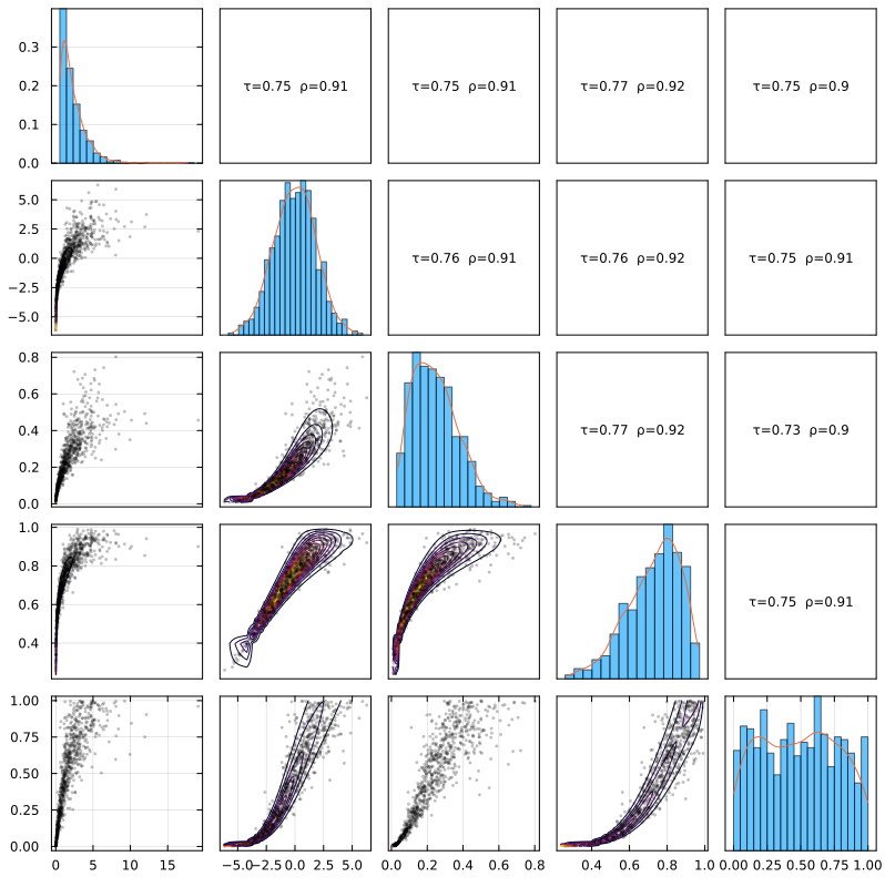
For a multivariate model, each off-diagonal panel shows one bivariate margin, the diagonal describes individual coordinates, and the upper triangle reports pairwise Kendall and Spearman coefficients. This representation is invariant to neither the selected scale nor the margins, except for the rank coefficients. It summarizes all pairs but does not prove that two multivariate models with the same pairwise margins have the same joint law.

Controlling resolution and presentation

The sample size n controls the scatterplots, while overlay_n controls the grid on which contours or surfaces are evaluated. Their roles are distinct: increasing n reveals the sampled cloud more densely; increasing overlay_n smooths the functional overlay at a cost proportional to roughly overlay_n^2.

Other useful choices are show_marginals, show_corr, bins, pts_alpha, marg_alpha, and show_axes. Standard Plots.jl attributes such as colors, themes, levels, size, and colorbar are forwarded to the recipe.

Density overlays are model-dependent

A PDF or log-PDF overlay is meaningful only when the displayed model has the corresponding ordinary density. Singular components and boundary behavior can make a scatterplot or CDF substantially more informative than a density contour.

A practical first look

Start with the default scatterplot, compare copula and Sklar scales when margins are present, and only then add a CDF or density overlay. A smoother contour cannot compensate for too few observations or an unsuitable model.

Bivariate views

Load Plots to activate the extension:

using Copulas
using Plots            # ensure recipes extension loads
using Distributions    # for marginals

Isolating the copula

A bivariate copula can be viewed as a sample alone or together with its CDF, density, or log-density. Comparing the four panels makes the distinction between probability accumulation and local density explicit:

gc = GaussianCopula(2, 0.75)
p1 = plot(gc; title="Default")
p2 = plot(gc, :pdf; title=":pdf")
p3 = plot(gc, :logpdf; title=":logpdf")
p4 = plot(gc, :cdf; title=":cdf")
plot(p1,p2,p3,p4; layout=(1,4), size=(1200,260))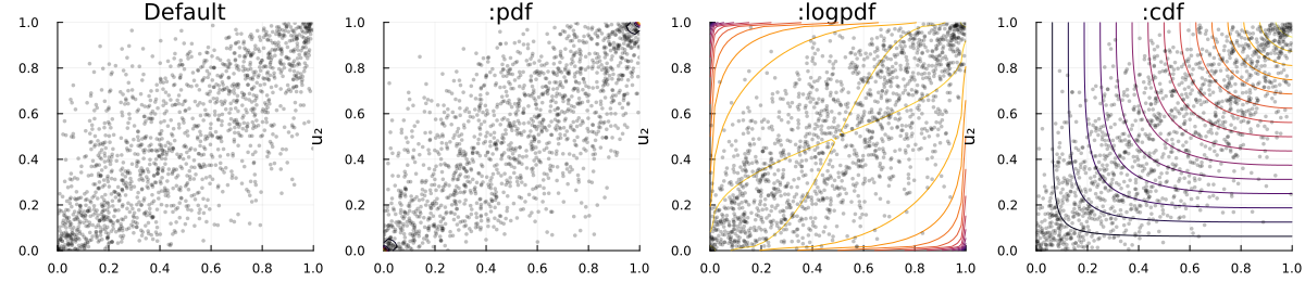

Restoring the margins

For a bivariate SklarDist, the default plot uses the copula scale and adds marginal summaries. This view keeps the dependence pattern comparable with a bare copula:

sd = SklarDist(GaussianCopula(2, 0.7), (Gamma(2,2), LogNormal(0.0,0.4)))
plot(sd)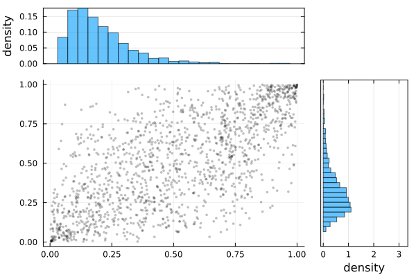

Setting scale=:sklar maps the same sample back to its original marginal units. Functional overlays are evaluated on the selected scale:

# Marginal scale with marginals
plot(sd, :logpdf; scale=:sklar)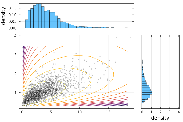

Marginal panels can be removed when the joint shape is the only object of interest:

q1 = plot(sd;          scale=:sklar, show_marginals=false, title="Default")
q2 = plot(sd, :pdf;    scale=:sklar, show_marginals=false, title=":pdf")
q3 = plot(sd, :logpdf; scale=:sklar, show_marginals=false, title=":logpdf")
q4 = plot(sd, :cdf;    scale=:sklar, show_marginals=false, title=":cdf")
plot(q1,q2,q3, q4; layout=(1,4), size=(1200,260))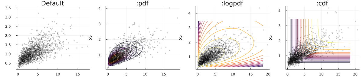

Surface views

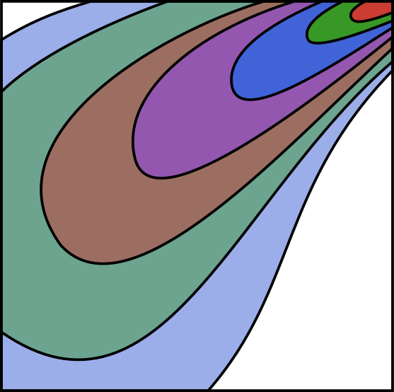
A surface emphasizes peaks, flat regions, and boundary behavior that may be hard to distinguish in contours:

fr = FrankCopula(2, 0.8)
s1 = plot(fr, :pdf; seriestype=:surface, title=":pdf")
s2 = plot(fr, :logpdf; seriestype=:surface, title=":logpdf")
s3 = plot(fr, :cdf; seriestype=:surface, title=":cdf")
plot(s1,s2,s3; layout=(1,3), size=(1800,560))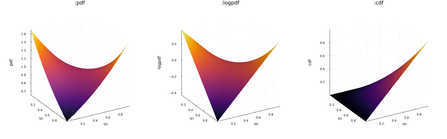

For a SklarDist, surfaces use the marginal scale by default:

sds = SklarDist(FrankCopula(2, 0.8), (Gamma(2,2), LogNormal(0.0,0.5)))
ss1 = plot(sds, :pdf; seriestype=:surface, title=":pdf")
ss2 = plot(sds, :logpdf; seriestype=:surface, title=":logpdf")
ss3 = plot(sds, :cdf; seriestype=:surface, title=":cdf")
plot(ss1,ss2,ss3; layout=(1,3), size=(1800,560))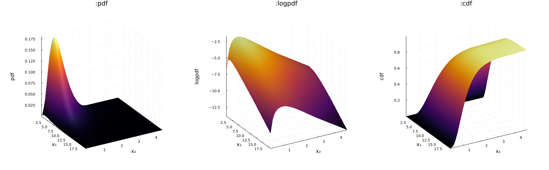

Set scale=:copula to remove the effect of the margins. Surface height and color both encode the selected function, so these plots are best used for exploration rather than quantitative comparison between panels with different scales.

Multivariate pairwise views

Remark: Pairwise evidence has limits

Pairwise panels are useful for locating heterogeneous dependence and suspicious margins. They cannot reveal interactions that exist only among three or more coordinates, and visual agreement in every panel is not a multivariate goodness-of-fit argument.

Copula models

A higher-dimensional copula is displayed as a pairwise matrix:

c5 = FrankCopula(5, 5.0)
plot(c5)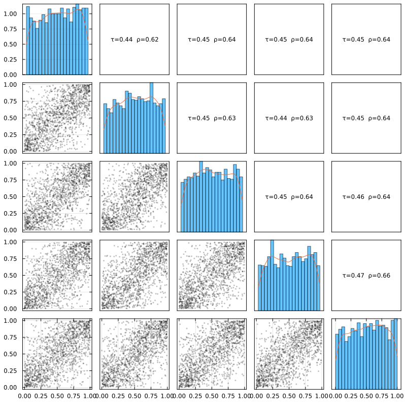

Overlays and annotations can be adjusted independently. For a busy matrix, removing the correlation labels or reducing the sample size often improves readability more than adding graphical detail:

c5 = FrankCopula(5, 12.0)
plot(c5, :pdf; show_corr=false, n=1200, overlay_n=70, pts_alpha=0.30, bins=30)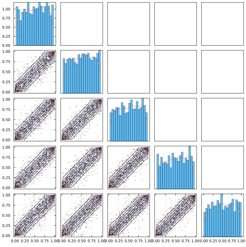

Sklar distributions

On the copula scale, heterogeneous margins no longer obscure differences in pairwise dependence:

SD5 = SklarDist(ClaytonCopula(5, 6.0), (Gamma(1,2), Normal(0,2), Beta(2,6), Beta(6,2), Uniform()))
plot(SD5, :pdf; n=800, overlay_n=60, pts_alpha=0.30, bins=28)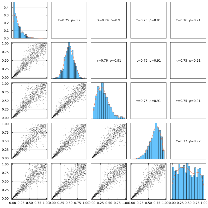

The number of sampled points and histogram bins should reflect the purpose of the plot. Small values are appropriate for a quick diagnostic; larger values reduce visual noise but increase rendering time:

plot(SD5; n=400, bins=12, show_corr=true)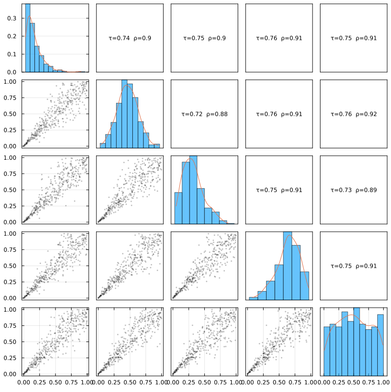

Finally, the Sklar scale restores the original units and marginal shapes:

plot(SD5, :pdf; scale=:sklar, n=800, bins=28)