Fitting from censored observations

Censoring is attached to observations, not to the copula itself. Its likelihood must therefore combine densities for observed coordinates with conditional survival probabilities for censored coordinates. This example builds that likelihood from the public conditioning API.

Consider two event times with different margins and different administrative right-censoring thresholds. To make the dependence model less conventional, we use an Archimax copula combining a Clayton generator with a Galambos tail.

using Copulas, Distributions, Optim, Random

rng = Xoshiro(361)
margins = (Weibull(1.6, 2.0), LogNormal(0.2, 0.55))
true_copula = ArchimaxCopula{2}(
    Copulas.ClaytonGenerator(1.4),
    Copulas.GalambosTail(0.8),
)
joint = SklarDist(true_copula, margins)

n = 80
latent = rand(rng, joint, n)
thresholds = (2.2, 1.8)
observed = min.(latent, reshape(collect(thresholds), :, 1))
exact = latent .<= reshape(collect(thresholds), :, 1)
count.(eachrow(.!exact))

2-element Vector{Int64}:
 27
 27

For one observation, four likelihood contributions are possible. When only one coordinate is censored, condition supplies its conditional distribution. When both are censored, flipping both coordinates turns the joint upper-tail probability into an ordinary copula CDF.

function censored_loglikelihood(C, margins, x, exact)
    total = 0.0
    survival = SurvivalCopula(C, (1, 2))
    for k in axes(x, 2)
        u = ntuple(i -> cdf(margins[i], x[i, k]), 2)
        e1, e2 = exact[1, k], exact[2, k]

        if e1 && e2
            total += logpdf(C, collect(u))
            total += logpdf(margins[1], x[1, k])
            total += logpdf(margins[2], x[2, k])
        elseif e1
            total += logpdf(margins[1], x[1, k])
            total += logccdf(condition(C, 1, u[1]), u[2])
        elseif e2
            total += logpdf(margins[2], x[2, k])
            total += logccdf(condition(C, 2, u[2]), u[1])
        else
            total += logcdf(survival, 1 .- collect(u))
        end
    end
    return total
end

censored_loglikelihood (generic function with 1 method)

We now keep the Galambos parameter and the margins fixed and estimate the Clayton parameter. The same pattern can be extended to optimize all model and marginal parameters jointly.

objective(θ) = -censored_loglikelihood(
    ArchimaxCopula{2}(Copulas.ClaytonGenerator(θ), Copulas.GalambosTail(0.8)),
    margins,
    observed,
    exact,
)

result = optimize(objective, 0.05, 4.0)
θ̂ = Optim.minimizer(result)
fitted_copula = ArchimaxCopula{2}(
    Copulas.ClaytonGenerator(θ̂),
    Copulas.GalambosTail(0.8),
)
(θ̂ = θ̂, converged = Optim.converged(result), fitted = fitted_copula)

(θ̂ = 1.7437092987741865, converged = true, fitted = BB4Copula{2, Float64}(1.7437092987741865, 0.8))

The distinction between the four cases is essential. Replacing a marginal by Distributions.censored(margin, upper=threshold) would describe its univariate law, but evaluating the resulting SklarDist at the threshold would still use the joint density. It would not integrate over the unknown event time, as the conditional survival terms above do.

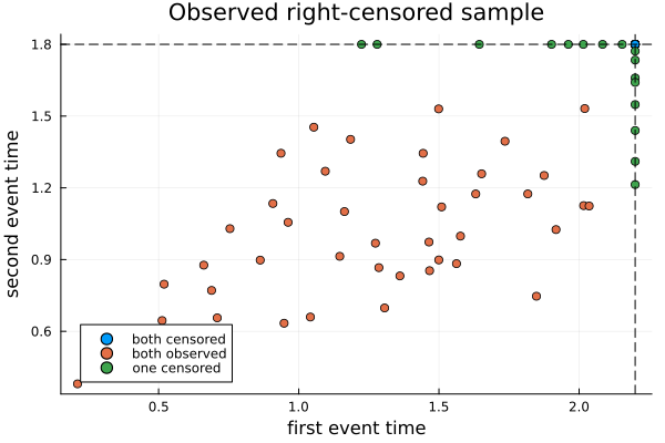
Finally, the observed sample makes the censoring geometry easy to see: censored coordinates accumulate on their respective thresholds.

using Plots

status = map(eachcol(exact)) do e
    e == [true, true] ? "both observed" :
    e == [false, false] ? "both censored" : "one censored"
end

scatter(
    observed[1, :], observed[2, :];
    group=status,
    xlabel="first event time",
    ylabel="second event time",
    title="Observed right-censored sample",
    markersize=4,
    legend=:bottomleft,
)
vline!([thresholds[1]]; color=:black, linestyle=:dash, label=false)
hline!([thresholds[2]]; color=:black, linestyle=:dash, label=false)