Nonparametric estimation of the radial law in Archimedean copulas

Introduction

This example recalls and implements a practical, nonparametric way to estimate the radial (mixing) distribution R that underlies a d-Archimedean copula by inverting a link between the kendall distribution and the radial part [41] [42], and applying this inversion to the empirical Kendall distribution. Suprisingly, a triangular recursion appears that maps empirical kendall atoms to radial atoms: see, in particular, [36]. We’ll:

• explain the idea,

• implement a small estimator,

• validate it visually on discrete and continuous radial laws,

• and compare original vs fitted copulas.

Definition: Radial distribution

For a d-Archimedean copula with generator $\phi$, there exists a nonnegative random variable $R$ (the radial law) such that

$$\phi (t)=\mathbb{E}\left[{(1-\frac{t}{R})}_{+}^{d-1}\right].$$

The empirical Kendall distribution of the copula sample carries enough information to reconstruct a discrete approximation of $R$ (up to scaling). That’s the key idea here.

Note that there exists other approaches at archimedean estimation:

• Parametric estimation fixes a generator family (Clayton, Gumbel, Frank, Joe, …) and estimates parameters by (pseudo-)likelihood, IFM, or moments such as inversion of Kendall’s $\tau$ [75]; [76]. Efficient but not nonparametric.

• Semiparametric approaches keep a parametric generator with nonparametric margins [77].

• Kendall-process methods, notably [78] for $d=2$, highlight the central role of the Kendall distribution. Extensions include settings with censoring [79].

Theoretical setup

Let $C$ be a $d$-dimensional Archimedean copula $(d\ge 2)$ with $d$-monotone generator $\phi$. By the Williamson representation [42]; [41], the random variable $R$ defined above exists and is unique up to scale.

If $\mathit{U}\sim C$, define the Kendall distribution

$$K_R(x)=\mathbb{P}(C(\mathit{U})\le x),x\in [0,1].$$

For empirical work, given a sample $\{{\mathit{U}}_i{\}}_{i=1}^n$ and the Deheuvels empirical copula $C_n$, the empirical Kendall distribution is

$${\hat{K}}_n(x)=\frac{1}{n}\sum _{i=1}^n\mathbf{1}\{C_n({\mathit{U}}_i)\le x\}.$$

When $R$ is discrete, $R=\sum _{j=1}^N{w}_j{\delta }_{r_j}$ with $0<r_1<\cdots <r_N$, the asociated generator writes

$${\phi }_R(t)=\sum _{j=1}^N{w}_j(1-\frac{t}{r_j}{)}_{+}^{d-1}.$$

Finally, it is known from [41] that when C is archimedean, the true kendall function writes

$$K_R(x)=\mathbb{P}({\phi }_R(R)\le u),$$

and therefore $K_R$ has jumps precisely at the points $x_j={\phi }_R(r_j)$ with masses $w_j$ when $R$ is discrete.

Proposed estimator (triangular inversion)

From the Kendall pseudo-sample $\{C_n({\mathit{U}}_i){\}}_{i=1}^n$, collect the distinct values and their empirical frequencies, defining

$$x_1>x_2>\cdots >x_N,w_j=\frac{1}{n}\sum _{i=1}^n\mathbf{1}\{C_n({\mathit{U}}_i)=x_j\},j=1,\dots ,N,$$

so that $\sum _{j=1}^N{w}_j=1$ and ${\hat{K}}_n(x)=\sum _{j=1}^N{w}_j\mathbf{1}\{x_j\le x\}$. Recover support points $0<r_1<\cdots <r_N$ by solving the system $x_j={\phi }_R(r_j)$. Because positive parts in ${\phi }_R$ switch on only when $r_j$ exceeds the evaluation point, the system is triangular:

$$\begin{array}{rl}& r_N:=1,\\ & r_{N-1}:=1-{\left(\frac{x_{N-1}}{w_N}\right)}^{1/(d-1)},\\ & \text{for }k=N-2,\dots ,1:x_k=\sum _{j=k+1}^N{w}_j(1-\frac{r_k}{r_j}{)}^{d-1},\end{array}$$

solved by monotone 1D root finding in $r_k\in [0,r_{k+1})$. The estimate is then

$$\hat{R}\sim \sum _{j=1}^N{w}_j{\delta }_{r_j}.$$

The associated generator ${\phi }_{\hat{R}}$ is continuous and piecewise polynomial between the recovered radii. We can prove existance and unicity of the obtained estimator, but convergence is still open since the representativity of the Kendall distribution is not certain in higher dimensions (see [36]).

Specificities when $d=2$

When $d=2$, powers reduce to 1 and closed forms appear. Let $A_k=\sum _{j=k+1}^N{w}_j$ and $B_k=\sum _{j=k+1}^N\frac{w_j}{r_j}$. Then the recursion gives

$$x_k=A_k-r_k{B}_k⟺r_k=\frac{A_k-x_k}{B_k}.$$

This closed form could be used directly (even if our code does not for the moment).

Implementation

We define a few helpers to visualize and validate the fitted model, and we now use the built-in EmpiricalGenerator as the estimator:

• simulate Archimedean copula samples from a given R,

• quick diagnostic plots, and

• optional visualization of φ_R for a discrete R.

using Distributions, StatsBase, Roots, QuadGK, Plots, Copulas


kendall_function(u::AbstractMatrix) = (W = Copulas._kendall_sample(u); t -> count(w -> w <= t, W) / length(W))

# Williamson d-transform φ_R for several R types
mk_ϕᵣ(R::DiscreteUnivariateDistribution, d) = let supp = support(R), w = pdf.(R, supp)
    t -> sum(wi * max(1 - t/x, 0)^(d-1) for (x, wi) in zip(supp, w))
end
mk_ϕᵣ(R::ContinuousUnivariateDistribution, d) = function(t)
    t == 0 && return 1 - Distributions.cdf(R, 0)
    val, = quadgk(x -> pdf(R, x) * (1 - t/x)^(d-1), t, Inf; rtol=1e-6)
    return val
end
mk_ϕᵣ(R::DiscreteNonParametric, d) = let supp = support(R), w = pdf.(R, support(R))
    t -> sum(wi * max(1 - t/r, 0)^(d-1) for (wi, r) in zip(w, supp))
end

# Simulate d×n Archimedean copula sample from a given radial R via simplex representation
function spl_cop(R, d::Int, n::Int)
    ϕᵣ = mk_ϕᵣ(R, d)
    S = -log.(rand(d, n))
    S ./= sum(S, dims=1)
    return ϕᵣ.(S .* rand(R, n)')
end

fit_empirical_generator(u::AbstractMatrix) = EmpiricalGenerator(u)

# Visual diagnostics: Kendall overlay + original vs simulated copula + (optional) histograms of R vs R̂
function diagnose_plots(u::AbstractMatrix, Rhat; R=nothing, logged=false)
    d, n = size(u)
    v = spl_cop(Rhat, d, n)
    K = kendall_function(u)
    ϕᵣ = mk_ϕᵣ(Rhat, d)
    supp = support(Rhat)
    a = [ϕᵣ.(r) for r in supp]
    w = pdf.(Rhat, supp)
    Kᵣ(x) = sum(w .* (a .< x))
    xs = range(0, 1; length=1001)
    # Compute difference series once and stabilize axis if essentially flat to avoid
    # PlotUtils warning: "No strict ticks found" (happens when span ~ 1e-16)
    diff_vals = K.(xs) .- Kᵣ.(xs)
    lo, hi = extrema(diff_vals)
    span = hi - lo
    # Threshold below which we consider the curve numerically flat
    if span < 1e-9
        # Center around mean (≈ mid of lo/hi) and impose a symmetric small band
        mid = (lo + hi) / 2
        pad = max(span, 1e-9) # ensure non‑zero
        lo_plot = mid - pad
        hi_plot = mid + pad
        # Provide explicit ticks so PlotUtils doesn't search for strict ticks
        tickvals = (mid - pad, mid, mid + pad)
    p1 = plot(xs, diff_vals; title="K̂ₙ(x) - K_R̂(x)", xlabel="", ylabel="", legend=false,
          ylims=(lo_plot, hi_plot), yticks=collect(tickvals))
    else
        p1 = plot(xs, diff_vals; title="K̂ₙ(x) - K_R̂(x)", xlabel="", ylabel="", legend=false)
    end
    p2 = plot(xs, xs .- K.(xs), label="x - K̂ₙ(x)", title="x - K̂ₙ(x) vs x - K_R̂(x)", xlabel="", ylabel="")
    plot!(p2, xs, xs .- Kᵣ.(xs), label="x - K_R̂(x)")

    p3 = scatter(u[1, :], u[2, :], title="Original sample (first two dims)", xlabel="", ylabel="",
                 alpha=0.25, msw=0, label=nothing)
    p4 = scatter(v[1, :], v[2, :], title="Simulated from R̂ (first two dims)", xlabel="", ylabel="",
                 alpha=0.25, msw=0, label=nothing)

    plots_list = [p1, p3, p2, p4]
    lay, sz = (2, 2), (1100, 800)

    if !isnothing(R)
        r1 = rand(Rhat, 10*n)
        r2 = rand(R, 10*n)
        ttl1, ttl2 = "R̂ histogram", "R histogram"
        if logged
            r1 .= log.(r1); r2 .= log.(r2)
            ttl1, ttl2 = "log(R̂) histogram", "log(R) histogram"
        end
        p6 = histogram(r1, title=ttl1, xlabel="", ylabel="", label=nothing, normalize=:pdf)
        p5 = histogram(r2, title=ttl2, xlabel="", ylabel="", label=nothing, normalize=:pdf)
        plots_list = [p1, p3, p5, p2, p4, p6]
        lay, sz = (2, 3), (1100, 700)
    end

    plot(plots_list...; layout=lay, size=sz)
end

# Optional: visualize φ_R(t) for a discrete radial law on a grid
function plot_phiR(R::DiscreteUnivariateDistribution, d::Int; tmax=maximum(support(R)), m=400)
    ϕᵣ = mk_ϕᵣ(R, d)
    ts = range(0, tmax; length=m)
    plot(ts, ϕᵣ.(ts), xlabel="t", ylabel="φ_R(t)", title="Williamson d-transform φ_R(t)", legend=false)
end

plot_phiR (generic function with 1 method)

Tip: Tip

Scale of R is not identifiable: φ_R depends on ratios t/R. We normalize the largest recovered radius to 1 without loss of generality.

Numerical illustrations

We now generate samples from several radial laws, fit R̂, and compare:

• Kendall function overlays,

• original vs simulated copula scatter,

• optionally histograms of R vs R̂ (or their logs for heavy tails).

Info: Sample sizes

To keep docs fast, we use modest sample sizes (n ≈ 1000–1500). Increase locally if you want smoother curves.

1) Dirac at 1 (lower-bound Clayton), d = 3

R = Dirac(1.0)
d, n = 3, 1000
u = spl_cop(R, d, n)
Ghat = EmpiricalGenerator(u)
Rhat = Copulas.𝒲₋₁(Ghat, d)
diagnose_plots(u, Rhat; R=R)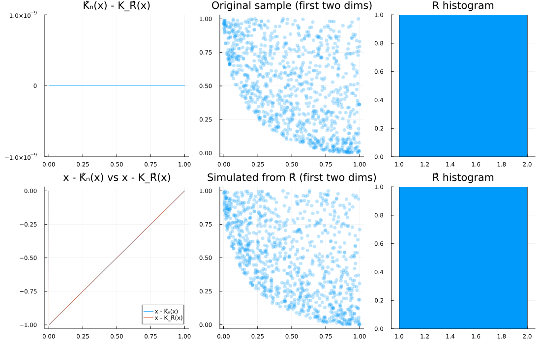

2) Mixture of point masses, d = 2

R = DiscreteNonParametric([1.0, 4.0, 8.0], fill(1/3, 3))
d, n = 2, 1000
u = spl_cop(R, d, n)
Ghat = EmpiricalGenerator(u)
Rhat = Copulas.𝒲₋₁(Ghat, d)
diagnose_plots(u, Rhat; R=R)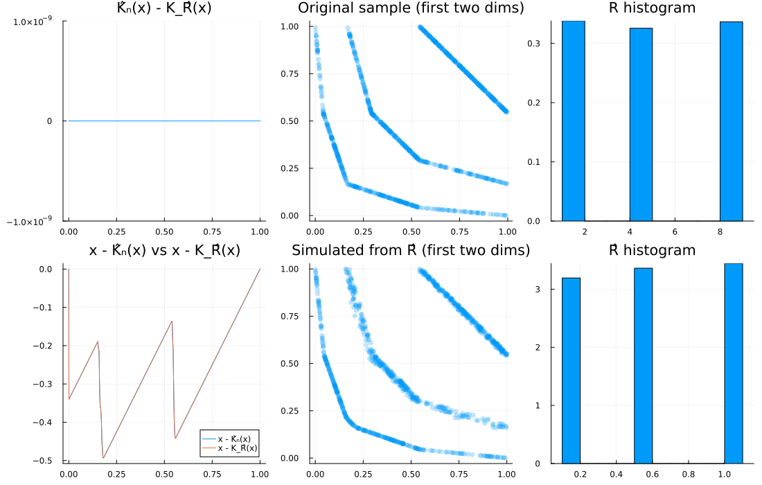

3) Mixture of point masses, d = 3

R = DiscreteNonParametric([1.0, 4.0, 8.0], fill(1/3, 3))
d, n = 3, 1000
u = spl_cop(R, d, n)
Ghat = EmpiricalGenerator(u)
Rhat = Copulas.𝒲₋₁(Ghat, d)
diagnose_plots(u, Rhat; R=R)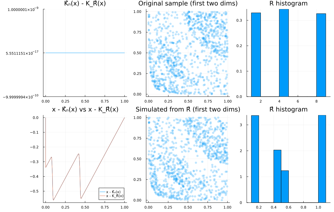

4) LogNormal(1, 3) (heavy tail), d = 10

R = LogNormal(1, 3)
d, n = 10, 1000
u = spl_cop(R, d, n)
Ghat = EmpiricalGenerator(u)
Rhat = Copulas.𝒲₋₁(Ghat, d)
diagnose_plots(u, Rhat; R=R, logged=true)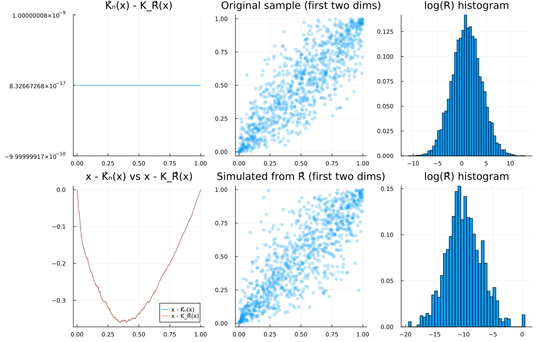

5) Pareto(1/2) (infinite mean), d = 10

R = Pareto(1.0, 1/2)
d, n = 10, 1000
u = spl_cop(R, d, n)
Ghat = EmpiricalGenerator(u)
Rhat = Copulas.𝒲₋₁(Ghat, d)
diagnose_plots(u, Rhat; R=R, logged=true)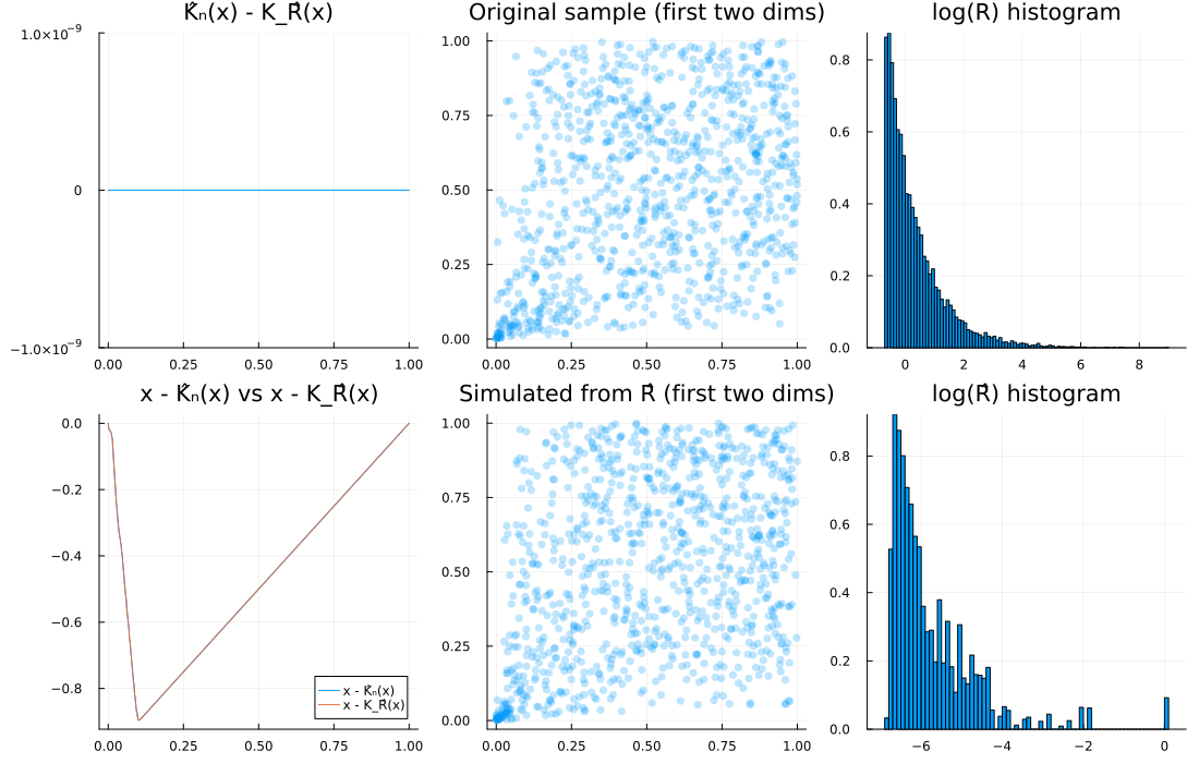

A quick look at ${\phi }_R$ {#A-quick-look-at-\varphi_R}

We can visualize ${\phi }_R$ for a discrete $\hat{R}$ to get intuition.

Rex = DiscreteNonParametric([0.2, 0.5, 1.0], [0.2, 0.3, 0.5])
plot_phiR(Rex, 3)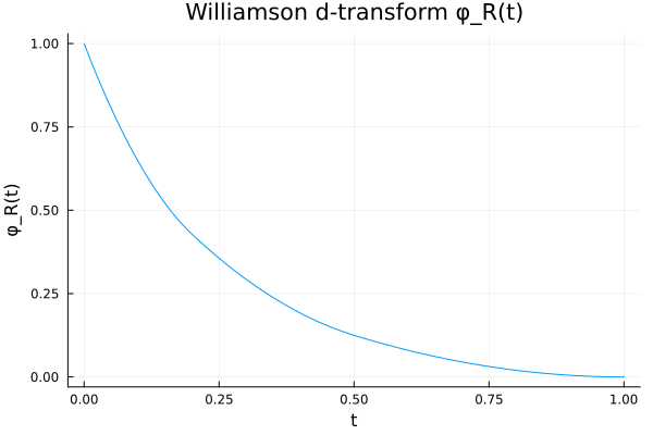

Discussion and caveats

• The fit is discrete even when the true $R$ is continuous: that’s expected. As $n$ grows, atoms densify in the bulk where Kendall jumps concentrate.

• Scale is not identifiable; we fix $r_N=1$.

• Very small weights can make the inversion numerically sensitive. Bootstrap CIs (not shown here) can complement delta-method formulas.

Liouville extension (remark)

The decoupling between the simplex and radial part allows the same idea to estimate radial parts of Liouville copulas. If $(D_1,\dots ,D_d)$ is Dirichlet and ${\phi }_s$ denotes the Williamson $s$-transform of $R$, then

$$C(\mathit{U})={\phi }_d(\sum _{i=1}^d{\phi }_{{\alpha }_i}^{-1}(U_i))={\phi }_d\left(R\sum _{i=1}^d{D}_i\right)={\phi }_d(R),$$

so Kendall atoms have the same form as in the Archimedean case, and the triangular inversion applies. Estimation of the Dirichlet parameters can be handled separately.

Once Liouville copulas are implemented in the package, we will probably use this method to fit them.

Appendix: Jacobian of the recursion (might be usefull for inference).

Define, for $k\in \{1,\dots ,N-1\}$ and $y\in [0,r_{k+1}]$,

$$g_k(y)=\sum _{j=k+1}^N{w}_j(1-\frac{y}{r_j}{)}^{d-1},g_k(r_k)=x_k.$$

Partial derivatives at the solution $r$ are

$$\begin{array}{rl}{A}_k& :=\frac{\partial g_k}{\partial y}(r_k)=-(d-1)\sum _{j=k+1}^N\frac{w_j}{r_j}(1-\frac{r_k}{r_j}{)}^{d-2},\\ B_{k,j}& :=\frac{\partial g_k}{\partial r_j}(r_k)=w_j(d-1)\frac{r_k}{r_j^2}(1-\frac{r_k}{r_j}{)}^{d-2},j\ge k+1,\\ C_{k,m}& :=\frac{\partial g_k}{\partial w_m}(r_k)=(1-\frac{r_k}{r_m}{)}^{d-1},m\ge k+1.\end{array}$$

Differentiating $g_k(r_k)=x_k$ gives triangular linear systems for the sensitivities $\partial r_k/\partial x_m$ and $\partial r_k/\partial w_m$:

$$\begin{array}{rl}{A}_k\frac{\partial r_k}{\partial x_m}+\sum _{j=k+1}^N{B}_{k,j}\frac{\partial r_j}{\partial x_m}& ={\mathbf{1}}_{\{m=k\}},\\ A_k\frac{\partial r_k}{\partial w_m}+\sum _{j=k+1}^N{B}_{k,j}\frac{\partial r_j}{\partial w_m}+C_{k,m}& =0.\end{array}$$

Solve downward in $k=N-1,\dots ,1$ with initialization $\partial r_N/\partial (\cdot )=0$.

The fitted generator $\hat{\phi }(t)=\sum _{j=1}^N{w}_j(1-t/r_j{)}_{+}^{d-1}$ has partials

$$\frac{\partial \phi (t)}{\partial r_j}=w_j(d-1)\frac{t}{r_j^2}(1-\frac{t}{r_j}{)}^{d-2},\frac{\partial \phi (t)}{\partial w_j}=(1-\frac{t}{r_j}{)}^{d-1}.$$

Combine with the chain rule to propagate variances via the delta method if needed.

References

1. C. Genest, J. Nešlehová and J. Ziegel. Inference in Multivariate Archimedean Copula Models. TEST 20, 223–256 (2011).

2. A. J. McNeil and J. Nešlehová. Multivariate Archimedean copulas, $d$-monotone functions and ${\ell }_1$-norm symmetric distributions. Annals of Statistics 37, 3059–3097 (2009).

3. R. E. Williamson. Multiply monotone functions and their Laplace transforms. Duke Mathematical Journal 23, 189–207 (1956).

4. A. J. McNeil, R. Frey and P. Embrechts. Estimation of copula models. Quantitative Risk Management: Concepts, Techniques and Tools, 235–284 (2008).

5. M. Hofert and A. J. McNeil. Nesting Archimedean copulas. Statistica Sinica 22, 441–477 (2012).

6. C. Genest, K. Ghoudi and L.-P. Rivest. A semiparametric estimation procedure of dependence parameters in multivariate families of distributions. Biometrika 82, 543–552 (1995).

7. C. Genest and L.-P. Rivest. Statistical inference procedures for bivariate Archimedean copulas. Journal of the American Statistical Association 88, 1034–1043 (1993).

8. M. Michaelides, H. Cossette and M. Pigeon. A non-parametric estimator for Archimedean copulas under flexible censoring scenarios and an application to claims reserving, arXiv preprint arXiv:2401.07724 (2024).