Empirical models

Pseudo-observations

Through the statistical process leading to the estimation of copulas, one usually observes the data and information on the marginals scale and not on the copula scale. This discrepancy between the observed information and the modeled distribution must be taken into account. A key concept is that of pseudo-observations.

Definition: Pseudo-observations

If $\mathit{x}\in {\mathbb{R}}^{N\times d}$ is an $N$-sample of a $d$-variate real-valued random vector $\mathit{X}$, then the pseudo-observations are the normalized ranks of the marginals of $\mathit{x}$, defined in the absence of ties as:

$$\mathit{u}\in [0,1{]}^{N\times d}:u_{i,j}=\frac{\mathrm{Rank}(x_{i,j},{\mathit{x}}_{\cdot ,j})}{N+1}=\frac{1}{N+1}\sum _{k=1}^N{\mathbb{1}}_{x_{k,j}\le x_{i,j}},$$

where $\mathrm{Rank}(y,\mathit{x})=\sum _{x_i\in \mathit{x}}{\mathbb{1}}_{x_i\le y}$.

With tied observations, the rank convention becomes part of the estimator. pseudos uses average ranks by default, matching the usual R and vinecopulib convention. The ties keyword also provides :first, :last, :min, :max, and :random; the latter accepts an explicit rng for reproducibility. These choices agree when margins are tie-free. A tie convention does not, on its own, make inference designed for continuous margins valid for discrete data.

In Copulas.jl, the function pseudos implements this transformation directly.

See the canonical Public API entry for pseudos.

Deheuvel's empirical copula

From these pseudo-observations, an empirical copula is defined and anlysed in [ DocumenterCitations.CitationSiteNode("deheuvels1979-cite-1")

] as follows:

Definition: Deheuvel's empirical copula

The empirical distribution function of the normalized ranks,

$${\hat{C}}_N(\mathit{u})=\frac{1}{N}\sum _{i=1}^N{\mathbb{1}}_{{\mathit{u}}_i\le \mathit{u}},$$

is called the empirical copula function.

Theorem: Exhaustivity and consistency

$${\hat{C}}_N$$

is an exhaustive estimator of $C$, and moreover for any normalizing constants $\{{\varphi }_N,N\in \mathbb{N}\}$ such that $\underset{N\to \mathrm{\infty }}{lim}{\varphi }_N\sqrt{N^{-1}\ln \ln N}=0$,

$$\underset{N\to \mathrm{\infty }}{lim}{\varphi }_N\underset{\mathit{u}\in [0,1{]}^d}{sup}|{\hat{C}}_N(\mathit{u})-C(\mathit{u})|=0\text{ a.s.}$$

$${\hat{C}}_N$$

then converges (weakly) to $C$, the true copula of the random vector $\mathit{X}$, when the number of observations $N$ goes to infinity.

The empirical copula is not a true copula

Despite its name, ${\hat{C}}_N$ is not a genuine copula on the full unit cube since its finite-sample margins are step functions rather than continuous uniforms. EmpiricalCopula keeps its historical Copula subtype for API compatibility, while algorithms that require exact uniform margins recognize this exception explicitly.

In the package, this copula is implemented as the EmpiricalCopula:

See the canonical Public API entry for EmpiricalCopula.

Passing it directly to SklarDist is allowed, but emits a warning: the resulting distribution generally does not have the requested margins. For a genuine copula model, smooth the empirical function with BetaCopula, a valid BernsteinCopula, or CheckerboardCopula. The direct construction remains useful when the intended model is the atomic empirical distribution transformed onto new coordinate scales; in that case pdf and logpdf report point masses rather than Lebesgue densities.

Conditionals and distortions

• Conditional distortions are defined by partial-derivative ratios. For the empirical copula, derivatives are stepwise; interpret results carefully near sample jumps.

• Conditional copulas are available through condition.

Visual: empirical copula from pseudo-observations

using Copulas, Distributions, Plots
# generate data with known dependence, then compute pseudo-observations
X = SklarDist(ClaytonCopula(2, 1.2), (Normal(), Beta(1, 4)))
x = rand(X, 1000)
Ĉ = EmpiricalCopula(x, pseudo_values=false)
plot(plot(first(params(X))), plot(Ĉ); layout=(1,2))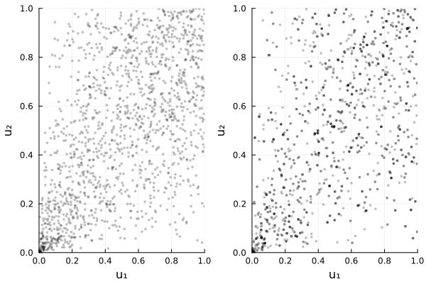

Beta copula

The empirical copula function is not a copula. An easy way to fix this problem is to smooth out the marginals with beta distribution functions. The Beta copula is thus defined and analysed in [ DocumenterCitations.CitationSiteNode("segers2017-cite-1")

] as follows:

Definition: Definition (Beta Copula)

Denoting $F_{n,r}(x)=\sum _{s=r}^n(\genfrac{}{}{0ex}{}{n}{s})x^s(1-x{)}^{n-s}$ as the distribution function of a $\mathrm{Beta}(r,n+1-r)$ random variable, the function

$${\hat{C}}_N^{\beta }:\mathit{x}\mapsto \frac{1}{N}\sum _{i=1}^N\prod _{j=1}^d{F}_{n,(N+1)u_{i,j}}(x_j)$$

is a genuine copula, called the Beta copula.

Property: Proximity of ${\hat{C}}_N$ and ${\hat{C}}_N^{\beta }$

$$\underset{\mathit{u}\in [0,1{]}^d}{sup}|{\hat{C}}_N(\mathit{u})-{\hat{C}}_N^{\beta }(\mathit{u})|\le d(\sqrt{\frac{\ln n}{n}}+\sqrt{\frac{1}{n}}+\frac{1}{n})$$

In the package, this copula is implemented as BetaCopula:

See the canonical Public API entry for BetaCopula.

Conditionals and distortions

• Conditional distortions support efficient evaluation and sampling.

• Conditional copulas are available through condition.

Performance notes

• Construction is O(d·n) after pseudo-observations are computed. Evaluation at a point uses O(d·n) basis lookups; consider subsampling for very large n.

Bernstein Copula

Bernstein copula are simply another smoothing of the empirical copula using Bernstein polynomials.

Mathematically, given a base copula $C$ and degrees $\mathit{m}=(m_1,\dots ,m_d)$, the (cdf) Bernstein copula is

$$B_{\mathit{m}}(C)(\mathit{u})=\sum _{s_1=0}^{m_1}\cdots \sum _{s_d=0}^{m_d}C(\frac{s_1}{m_1},\dots ,\frac{s_d}{m_d})\prod _{j=1}^d(\genfrac{}{}{0ex}{}{m_j}{s_j})u_j^{s_j}(1-u_j{)}^{m_j-s_j}.$$

It is a multivariate Bernstein polynomial approximation of $C$ on the uniform grid. Larger $m_j$ increase smoothness and accuracy at higher computational cost. When the base is an empirical copula built from $n$ tie-free observations, however, the result has exactly uniform margins if and only if every $m_j$ divides $n$ [ DocumenterCitations.CitationSiteNode("segers2017-cite-2")

]. BernsteinCopula rejects degrees that violate this condition instead of returning a multivariate distribution mislabeled as a copula. With m=nothing, it selects the largest divisor of $n$ no greater than $\lfloor n^{1/d}\rfloor$.

The divisibility restriction is specific to the empirical construction. Applying the Bernstein operator to a genuine copula preserves uniform margins for arbitrary positive degrees. Constructors nevertheless verify the resulting cell masses, so tied empirical ranks or numerically invalid base values cannot silently produce a non-copula.

In the package, this copula is implemented as BernsteinCopula:

See the canonical Public API entry for BernsteinCopula.

Conditionals and distortions

• Conditional distortions are obtained from the Bernstein grid conditioned on ${\mathit{u}}_J$ and support evaluation and sampling.

• Conditional copulas are available through condition.

Performance notes

• Complexity grows with the grid size ∏_j (m_j+1) for cdf and ∏_j m_j for pdf. In higher dimensions, keep m small or prefer the 2D specialized paths provided.

• The constructor tolerates floating-point roundoff in finite differences, but rejects materially negative cell masses or non-uniform margins.

Checkerboard Copulas

There are other nonparametric estimators of the copula function that are true copulas. Of interest to our work is the Checkerboard construction (see [ DocumenterCitations.CitationSiteNode("cuberos2019-cite-1")

, DocumenterCitations.CitationSiteNode("mikusinski2010-cite-1")

]), detailed below.

First, for any $\mathit{m}\in {\mathbb{N}}^d$, let $\{B_{\mathit{i},\mathit{m}},\mathit{i}<\mathit{m}\}$ be a partition of the unit hypercube defined by

$$B_{\mathit{i},\mathit{m}}=]\frac{\mathit{i}}{\mathit{m}},\frac{\mathit{i}+1}{\mathit{m}}].$$

Furthermore, for any copula $C$ (or more generally distribution function $F$), we denote ${\mu }_C$ (resp ${\mu }_F$) the associated measure. For example, for the independence copula $Pi$, ${\mu }_{\mathrm{\Pi }}(A)=\lambda (A\cup [\mathbf{0},\mathbf{1}])$ where $\lambda$ is the Lebesgue measure.

Definition: Empirical Checkerboard copulas

Let $\mathit{m}\in {\mathbb{N}}^d$. The $\mathit{m}$-Checkerboard copula ${\hat{C}}_{N,\mathit{m}}$, defined by

$${\hat{C}}_{N,\mathit{m}}(\mathit{x})={\mathit{m}}^{\mathbf{1}}\sum _{\mathit{i}<\mathit{m}}{\mu }_{{\hat{C}}_N}(B_{\mathit{i},\mathit{m}}){\mu }_{\mathrm{\Pi }}(B_{\mathit{i},\mathit{m}}\cap [0,\mathit{x}]),$$

is a genuine copula as soon as $m_1,...,m_d$ all divide $N$.

Property: Consistency of ${\hat{C}}_{N,\mathit{m}}$

If all $m_1,...,m_d$ divide $N$,

$$\underset{\mathit{u}\in [0,1{]}^d}{sup}|{\hat{C}}_{N,\mathit{m}}(\mathit{u})-C(\mathit{u})|\le \frac{d}{2m}+{\mathcal{O}}_{\mathbb{P}}\left(n^{-1/2}\right).$$

This copula is called Checkerboard, as it fills the unit hypercube with hyperrectangles of same shapes $B_{\mathit{i},\mathit{m}}$, conditionally on which the distribution is uniform, and the mixing weights are the empirical frequencies of the hyperrectangles.

It can be noted that there is no need for the hyperrectangles to be filled with a uniform distribution (${\mu }_{\mathrm{\Pi }}$), as soon as they are filled with copula measures and weighted according to the empirical measure in them (or to any other copula). The direct extension is then the more general patchwork copulas, whose construction is detailed below.

Denoting $B_{\mathit{i},\mathit{m}}(\mathit{x})=B_{\mathit{i},\mathit{m}}\cap [0,\mathit{x}]$, we have :

$$\begin{array}{rl}{m}^d{\mu }_{\mathrm{\Pi }}(B_{\mathit{i},\mathit{m}}\cap [0,\mathit{x}])& =\frac{{\mu }_{\mathrm{\Pi }}(B_{\mathit{i},\mathit{m}}\cap [0,\mathit{x}])}{{\mu }_{\mathrm{\Pi }}(B_{\mathit{i},\mathit{m}})}\\ & =\frac{{\mu }_{\mathrm{\Pi }}(B_{\mathit{i},\mathit{m}}(\mathit{x}))}{{\mu }_{\mathrm{\Pi }}(B_{\mathit{i},\mathit{m}})}\\ & ={\mu }_{\mathrm{\Pi }}(\mathit{m}{B}_{\mathit{i},\mathit{m}}(\mathit{x}))\end{array}$$

where we intend $\mathit{m}]\mathit{a},\mathit{b}]=]\mathit{m}\mathit{a},\mathit{m}\mathit{b}]$ (products between vectors are componentwise).

This allows for an easy generalization in the framework of patchwork copulas [ DocumenterCitations.CitationSiteNode("durante2012-cite-1")

– DocumenterCitations.CitationSiteNode("durante2015-cite-1")

]:

Definition: Patchwork copulas

Let $\mathit{m}\in {\mathbb{N}}^d$ all divide $N$, and let $\mathcal{C}=\{C_{\mathit{i}},\mathit{i}<\mathit{m}\}$ be a given collection of copulas. The distribution function:

$${\hat{C}}_{N,\mathit{m},\mathcal{C}}(\mathit{x})=\sum _{\mathit{i}<\mathit{m}}{\mu }_{{\hat{C}}_N}(B_{\mathit{i},\mathit{m}}){\mu }_{C_{\mathit{i}}}(\mathit{m}{B}_{\mathit{i},\mathit{m}}(\mathit{x}))$$

is a copula.

In fact, replacing ${\hat{C}}_N$ by any copula in the patchwork construct still yields a genuine copula, with no more conditions that all components of $\mathit{m}$ divide $N$. The Checkerboard grids are practical in the sense that computations associated to a Checkerboard copula can be really fast: if the grid is large, the number of boxes is small, and otherwise if the grid is very refined, many boxes are probably empty. On the other hand, the grid is fixed a priori, see [ DocumenterCitations.CitationSiteNode("laverny2020-cite-1")

] for a construction with an adaptive grid.

Convergence results for this kind of copulas can be found in [ DocumenterCitations.CitationSiteNode("durante2015-cite-2")

], with a slightly different parametrization.

In the package, this copula is implemented as CheckerboardCopula:

See the canonical Public API entry for CheckerboardCopula.

Conditionals and distortions

• Conditioning on one coordinate uses the corresponding histogram slice.

• Conditioning on several coordinates preserves the checkerboard semantics on the remaining axes and renormalizes the relevant cell probabilities.

Performance notes

• Construction cost scales with sample size but stores only occupied boxes (sparse). CDF evaluation is O(#occupied boxes) at query time.

• For large n choose coarser m to reduce occupied boxes; for small n a finer grid is possible but may leave many empty boxes.

Empirical Extreme-Value copula

In addition to the empirical, beta, Bernstein and checkerboard constructions, Copulas.jl provides a nonparametric extreme-value estimator through EmpiricalEVCopula. It accepts a sample in the usual $d\times n$ layout and returns an ExtremeValueCopula whose tail is estimated from the pseudo-observations.

The same public constructor selects a dimension-appropriate representation:

• in $d=2$, EmpiricalEVTail estimates the scalar Pickands function using the Pickands, CFG, or OLS-intercept estimator;

• in $d\ge 3$, EmpiricalEVMultivariateTail builds a multivariate Pickands pilot and projects it onto a finite discrete spectral measure. The projection enforces a valid stable tail dependence function and provides an exact spectral sampler for the fitted model.

Here is a complete multivariate workflow:

using Copulas, Distributions, Random

rng = Xoshiro(42)
Ctrue = LogCopula{3}(2.0)
U = rand(rng, Ctrue, 150)

Chat = EmpiricalEVCopula{3}(U; method=:ols, degree=3)
(cdf(Chat, [0.4, 0.6, 0.8]), size(rand(rng, Chat, 100)))

(0.3346478302140466, (3, 100))

The runtime-dimension and inferred-dimension forms are equivalent:

Chat_runtime = EmpiricalEVCopula(3, U; method=:ols, degree=3)
Chat_inferred = EmpiricalEVCopula(U; method=:ols, degree=3)

The estimator is also available through the common fitting interface:

Chat_fit = fit(Copulas.ExtremeValueCopula, U; method=:ols, degree=3)

The projected multivariate model may contain singular components. Therefore cdf and rand are supported, but a global Lebesgue pdf is deliberately not defined. See Extreme Value copulas for the STDF theory, the projection references, and the complete list of EV families.

See the canonical Public API entries for EmpiricalEVTail, EmpiricalEVMultivariateTail.

Empirical Archimedean generator (Kendall inversion)

Beyond copula estimators, we also provide a nonparametric estimator of a $d$-Archimedean generator from data, based on the empirical Kendall distribution following [ DocumenterCitations.CitationSiteNode("genest2011a-cite-1")

]. For a $d$-Archimedean copula with generator $\phi$, there exists a nonnegative random variable $R$ (the radial law) such that

$$\phi (t)=\mathbb{E}[(1-t/R{)}_{+}^{d-1}].$$

Approximating the (unknown) $R$ by a discrete measure $\hat{R}=\sum _j{w}_j{\delta }_{r_j}$ yields a piecewise-polynomial generator

$$\hat{\phi }(t)=\sum _j{w}_j(1-t/r_j{)}_{+}^{d-1}.$$

The radii and weights are recovered from the empirical Kendall distribution via a triangular recursion (see the example page for details), and the resulting generator is exposed as EmpiricalGenerator.

Usage:

• Build from d×n pseudo-observations: Ĝ = EmpiricalGenerator(u; pseudo_values=true). For raw data, use pseudo_values=false.

• Use directly in an Archimedean copula: Ĉ = ArchimedeanCopula(d, Ĝ)

• Access the fitted radial law: R̂ = 𝒲₋₁(Ĝ, d)

See the canonical Public API entry for EmpiricalGenerator.

Performance notes

• The Kendall sample computation is currently O(n^2) in the number of observations. For large n, future versions may switch to Fenwick-tree–based sweeps to reach ~O(n log n) in bivariate cases and ~O(n log^{d-1} n) for higher d.

See This example page for more details and example usages.

Available models

EmpiricalCopula

For observations ${\mathit{U}}_1,\dots ,{\mathit{U}}_n$, the empirical CDF is $C_n(\mathit{u})=n^{-1}\sum _i\mathbf{1}\{{\mathit{U}}_i\le \mathit{u}\}$. Construct it from a $d\times n$ matrix with EmpiricalCopula(U; pseudo_values=true), EmpiricalCopula{d}(U; ...), or EmpiricalCopula(d, U; ...); use pseudo_values=false for raw observations.

BernsteinCopula

The Bernstein copula applies the multivariate Bernstein polynomial displayed above to a base copula or empirical sample. The integer or tuple m gives the polynomial degrees. Use BernsteinCopula(C; m=10), BernsteinCopula(U; m=10), or the corresponding {d} / (d, ...) forms.

CheckerboardCopula

The checkerboard copula assigns empirical probability $w_k$ to each regular grid cell and is uniform within that cell. Thus its density there is $w_k\prod _j{m}_j$ and its CDF is the multilinear cell-overlap interpolation. Use CheckerboardCopula(U; m=nothing, pseudo_values=true) or the corresponding {d} / (d, ...) forms. Every $m_j$ must divide the sample size.

BetaCopula

The empirical beta copula replaces each rank indicator by the CDF of a $\mathrm{Beta}(R_{ij},n+1-R_{ij})$ variable, as defined above. Build it from a $d\times n$ data matrix with BetaCopula(U), BetaCopula{d}(U), or BetaCopula(d, U).

EmpiricalEVCopula

This estimator projects an empirical extreme-value estimate onto a valid Pickands function in dimension two or a valid spectral/STDF model in higher dimension. Use EmpiricalEVCopula(U; method=:ols), EmpiricalEVCopula{d}(U; method=:ols), or EmpiricalEVCopula(d, U; method=:ols); degree controls the multivariate projection basis.

See the canonical Public API for all estimator options and validation.

References

1. C. Genest, J. Nešlehová and J. Ziegel. Inference in Multivariate Archimedean Copula Models. TEST 20, 223–256 (2011).

2. P. Deheuvels. La Fonction de Dépendance Empirique et Ses Propriétés. Académie Royale de Belgique. Bulletin de la Classe des Sciences 65, 274–292 (1979).

3. J. Segers, M. Sibuya and H. Tsukahara. The Empirical Beta Copula. Journal of Multivariate Analysis 155, 35–51 (2017).

4. A. Cuberos, E. Masiello and V. Maume-Deschamps. Copulas Checker-Type Approximations: Application to Quantiles Estimation of Sums of Dependent Random Variables. Communications in Statistics - Theory and Methods 49, 3044–3062 (2020).

5. P. Mikusiński and M. D. Taylor. Some Approximations of N-Copulas. Metrika 72, 385–414 (2010).

6. F. Durante, E. Foscolo, J. A. Rodríguez-Lallena and M. Úbeda-Flores. A Method for Constructing Higher-Dimensional Copulas. Statistics 46, 387–404 (2012).

7. F. Durante, J. Fernández Sánchez and C. Sempi. Multivariate Patchwork Copulas: A Unified Approach with Applications to Partial Comonotonicity. Insurance: Mathematics and Economics 53, 897–905 (2013).

8. F. Durante, J. Fernández-Sánchez, J. J. Quesada-Molina and M. Úbeda-Flores. Convergence Results for Patchwork Copulas. European Journal of Operational Research 247, 525–531 (2015).

9. O. Laverny. Empirical and Non-Parametric Copula Models with the Cort R Package. Journal of Open Source Software 5, 2653 (2020).