Copulas and Sklar Distributions

This section gives some general definitions and tools about dependence structures, multivariate random vectors and copulas. Along this journey through the mathematical theory of copulas, we link to the rest of the documentation for more specific and detailed arguments on particular points, or simply to the technical documentation of the actual implementation. The interested reader can take a look at the standard books on the subject [ DocumenterCitations.CitationSiteNode("joe1997-cite-1")

– DocumenterCitations.CitationSiteNode("joe2014-cite-1")

] or more recently [ DocumenterCitations.CitationSiteNode("mai2017-cite-1")

– DocumenterCitations.CitationSiteNode("grosser2021-cite-1")

].

We start here by defining a few concepts about multivariate random vectors, dependence structures and copulas.

Reminder on multivariate random vectors

Consider a real valued random vector $\mathit{X}=(X_1,...,X_d):\mathrm{\Omega }\to {\mathbb{R}}^d$. The random variables $X_1,...,X_d$ are called the marginals of the random vector $\mathit{X}$.

Constructing random variables in Julia via Distributions.jl

Recall that you can construct random variables in Julia by the following code :

using Distributions
X₁ = Normal()       # A standard Gaussian random variable
X₂ = Gamma(2,3)     # A Gamma random variable
X₃ = Pareto(1)      # A Pareto random variable with infinite variance.
X₄ = LogNormal(0,1) # A Lognormal random variable

We refer to Distributions.jl's documentation for more details on what you can do with these objects. We assume here that you are familiar with their API.

The probability distribution of the random vector $\mathit{X}$ can be characterized by its distribution function $F$:

$$\begin{array}{rl}F(\mathit{x})& =\mathbb{P}(\mathit{X}\le \mathit{x})\\ & =\mathbb{P}(\mathrm{\forall }i\in \{1,...,d\},X_i\le x_i).\end{array}$$

For a function $F$ to be the distribution function of some random vector, it should be $d$-increasing, right-continuous and left-limited. For $i\in \{1,...,d\}$, the random variables $X_1,...,X_d$, called the marginals of the random vector, also have distribution functions denoted $F_1,...,F_d$ and defined by :

$$F_i(x_i)=F(+\mathrm{\infty },...,+\mathrm{\infty },x_i,+\mathrm{\infty },...,+\mathrm{\infty }).$$

Note that the range $\mathrm{Ran}(F)$ of a distribution function $F$, univariate or multivariate, is always contained in $[0,1]$. When the random vector or random variable is absolutely continuous with respect to (w.r.t.) the Lebesgue measure restricted to its domain, the range is exactly $[0,1]$. When the distribution is discrete with $n$ atoms, the range is a finite set of $n+1$ values in $[0,1]$.

Copulas and Sklar's Theorem

There is a fundamental functional link between the function $F$ and its marginals $F_1,...,F_d$. This link is expressed by the mean of copulas.

Definition: Copula

A copula, usually denoted $C$, is the distribution function of a random vector with marginals that are all uniform on $[0,1]$, i.e.

$$C_i(u)=u{\mathbb{1}}_{u\in [0,1]}\text{ for all }i\in 1,...,d.$$

Vocabulary

In this documentation but more largely in the literature, the term Copula refers both to the random vector and its distribution function. Usually, the distinction is clear from context.

You may define a copula object in Julia by simply calling its constructor:

using Copulas
d = 3 # The dimension of the model
θ = 7 # Parameter
C = ClaytonCopula(d,7) # A 3-dimensional clayton copula with parameter θ = 7.

ClaytonCopula{3, Float64}(7.0,)

When the dimension is known at compile time, the equivalent ClaytonCopula{3}(7) form makes it explicit as the first type parameter. This dimension-fixed form is useful in performance-sensitive or generic code because its return type can be inferred without relying on the runtime value of d. The convenient ClaytonCopula(d, 7) form remains appropriate for interactive use and for dimensions that are only known at runtime.

This object is a random vector, and behaves exactly as you would expect a random vector from Distributions.jl to behave: you may sample it with rand(C,100), compute its pdf or cdf with pdf(C,x) and cdf(C,x), etc:

u = rand(C,10)

3×10 Matrix{Float64}:
 0.156233  0.590796  0.794556  0.905754  …  0.154626  0.0648702  0.684927
 0.233367  0.605343  0.655051  0.71973      0.147377  0.0606048  0.670528
 0.142031  0.649545  0.675442  0.909068     0.13624   0.0647847  0.566624

cdf(C,u)

10-element Vector{Float64}:
 0.1334839670856987
 0.5242537839902345
 0.5949131248899822
 0.7016493825934105
 0.006199925196818117
 0.11715428034991009
 0.83319846797161
 0.12349160454736335
 0.05398159066956455
 0.5329567204594363

You can also plot it:

using Plots
plot(C, :logpdf)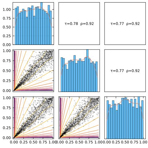

See the visualizations page for details on the visualisations tools. It’s often useful to get an intuition by looking at scatter plots.

Example: Independence

To give another example, the function

$$\mathrm{\Pi }:\mathit{x}\mapsto \prod _{i=1}^d{x}_i={\mathit{x}}^{\mathbf{1}}$$

is a copula, corresponding to independent random vectors.

This copula can be constructed using the IndependentCopula(d) syntax as follows:

Π = IndependentCopula(d) # A 4-variate independence structure.

One of the reasons that makes copulas so useful is the bijective map from the Sklar Theorem [ DocumenterCitations.CitationSiteNode("sklar1959-cite-1")

]:

Theorem: Sklar (1959)

For every random vector $\mathit{X}$, there exists a copula $C$ such that

$$\mathrm{\forall }\mathit{x}\in {\mathbb{R}}^d,F(\mathit{x})=C(F_1(x_1),...,F_d(x_d)).$$

The copula $C$ is uniquely determined on $\mathrm{Ran}(F_1)\times ...\times \mathrm{Ran}(F_d)$, where $\mathrm{Ran}(F_i)$ denotes the range of the function $F_i$. In particular, if all marginals are absolutely continuous, $C$ is unique.

This result allows to decompose the distribution of $\mathit{X}$ into several components: the marginal distributions on one side, and the copula on the other side, which governs the dependence structure between the marginals. This object is central in our work, and therefore deserves a moment of attention.

We can then leverage the Sklar theorem to construct multivariate random vectors from a copula-marginals specification. The implementation we have of this theorem allows building multivariate distributions by specifying separately their marginals and dependence structures as follows:

X₁, X₂, X₃ = Gamma(2,3), Pareto(), LogNormal(0,1) # Marginals
D = SklarDist(C, (X₁,X₂,X₃)) # The final distribution, using the previous copula C.
plot(D, scale=:sklar)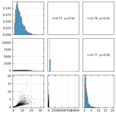

The obtained multivariate random vector object are genuine multivariate random vector following the Distributions.jl API. They can be sampled (rand()), and their probability density function and distribution function can be evaluated (respectively pdf and cdf), etc:

x = rand(D,10)
p = pdf(D, x)
l = logpdf(D, x)
c = cdf(D, x)
[x' p l c]

10×6 Matrix{Float64}:
  5.49973  2.13572  1.26326    0.0718217    -2.63357   0.473109
  4.38749  2.69773  0.974383   0.0206236    -3.88132   0.406802
  4.09144  2.03723  1.10067    0.039999     -3.2189    0.381736
  3.98866  1.42602  0.751423   0.268927     -1.31332   0.286662
  3.75914  1.84643  0.599948   0.101784     -2.2849    0.290693
 11.3984   7.71231  2.07999    0.000488116  -7.62496   0.728274
  1.11823  1.05295  0.178606  26.992         3.29554   0.0401515
  2.15528  1.15983  0.319287   5.32515       1.67244   0.117184
  2.85127  1.27613  0.451497   2.75471       1.01331   0.189676
  3.08692  1.28678  0.497786   1.72922       0.547672  0.205238

Sklar's theorem can be used the other way around (from the marginal space to the unit hypercube): this is, for example, what pseudos does by computing normalized ranks.

Independent random vectors

Distributions.jl provides the product_distribution function to create independent random vectors with given marginals. product_distribution(args...) is essentially equivalent to SklarDist(IndependentCopula(d), args), but our approach generalizes to other dependence structures.

Copulas are bounded functions with values in [0,1] since they correspond to probabilities. But their range can be bounded more precisely, and [ DocumenterCitations.CitationSiteNode("lux2017-cite-1")

] gives us:

Property: Fréchet-Hoeffding bounds

For all $\mathit{x}\in [0,1{]}^d$, every copula $C$ satisfies :

$$⟨\mathbf{1},\mathit{x}-1+d^{-1}{⟩}_{+}\le C(\mathit{x})\le min\mathit{x},$$

where $y_{+}=max(0,y)$.

The function $M:\mathit{x}\mapsto min\mathit{x}$, called the upper Fréchet-Hoeffding bound, is a copula. The function $W:\mathit{x}\mapsto ⟨\mathbf{1},\mathit{x}-1+d^{-1}{⟩}_{+}$, called the lower Fréchet-Hoeffding bound, is on the other hand a copula only when $d=2$. These two copulas can be constructed through MCopula(d) and WCopula(2).

The upper Fréchet-Hoeffding bound corresponds to the case of comonotone random vector: a random vector $\mathit{X}$ is said to be comonotone, i.e., to have copula $M$, when each of its marginals can be written as a non-decreasing transformation of the same random variable (say with $\mathcal{U}([0,1])$ distribution). This is a simple but important dependence structure. See e.g.,[ DocumenterCitations.CitationSiteNode("kaas2002-cite-1")

, DocumenterCitations.CitationSiteNode("hua2017-cite-1")

] on this particular copula.

Here is a plot of the independence, a positive dependence (Clayton), and the Fréchet bounds in bivariate cases. You can visualize the strong alignment for M and the anti-diagonal pattern for W.

p1 = plot(IndependentCopula(2), title="IndependentCopula(2)")
p2 = plot(ClaytonCopula(2, 3.0), title="ClaytonCopula(2, 3.0)")
p3 = plot(MCopula(2), title="MCopula(2)")
p4 = plot(WCopula(2), title="WCopula(2)")
plot(p1,p2,p3,p4; layout=(2,2), size=(800,600))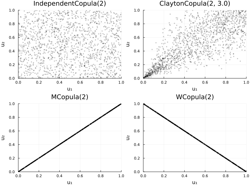

Since copulas are distribution functions, like distribution functions of real-valued random variables and random vectors, there exists classical and useful parametric families of copulas (we already saw the Clayton family). You can browse the available families in this package in the Bestiary. Like any families of random variables or random vectors, copulas are fittable on empirical data.

A tour of the main API

The public API of Copulas.jl is quite small and easy to expose on a simple example, which is what we will do right now.

Copulas and SklarDist

The most important objects of the package are of course copulas as sklar distributions. Both of these objects follow the Distributions.jl's API, and so you can construct, sample, and evaluate copulas as standard Distributions.jl objects:

using Copulas, Distributions, Random, StatsBase
C = ClaytonCopula(3, 2.0)
u = rand(C, 5)
Distributions.loglikelihood(C, u)

2.737822013183484

X₁, X₂, X₃ = Gamma(2,3), Beta(1,5), LogNormal(0,1)
C2 = GumbelCopula(3, 1.7)
D = SklarDist(C2, (X₁, X₂, X₃))
rand(D, 3)
pdf(D, rand(3))

1.1993991961116367e-5

Basic dependence metrics.

Basic dependence summaries available on copulas, whatever their dimension d:

multivariate_stats = (
    kendall_tau = Copulas.τ(C),
    spearm_rho = Copulas.ρ(C),
    blomqvist_beta = Copulas.β(C),
    gini_gamma = Copulas.γ(C),
    entropy_iota = Copulas.ι(C),
    lower_tail_dep = Copulas.λₗ(C),
    upper_tail_dep = Copulas.λᵤ(C)
)

(kendall_tau = 0.5, spearm_rho = 0.6822338340468788, blomqvist_beta = 0.5118578920369089, gini_gamma = 0.5317438932925356, entropy_iota = -0.9597434014371774, lower_tail_dep = 0.5773502691896282, upper_tail_dep = 0.0)

The entropy measure ι requires an ordinary Lebesgue density and is therefore not defined for purely singular copulas. The other summaries are available for continuous, mixed, and singular models through their documented generic or specialized implementations.

The same functions accept a d×n matrix, with variables in rows and observations in columns, and provide sample versions of these quantities. Since these statistics are especially common in the bivariate case, the following functions return matrices of pairwise dependence measures:

StatsBase.corkendall(C)
StatsBase.corspearman(C)
Copulas.corblomqvist(C)
Copulas.corgini(C)
Copulas.corentropy(C)
Copulas.corlowertail(C)
Copulas.coruppertail(C)

For a data matrix, these pairwise functions follow the StatsBase convention: observations in rows and variables in columns (n×d), unlike the scalar multivariate functions above.

Measure function

A measure function gives the measure of hypercubes from any copula as follows:

Copulas.measure(C, (0.1,0.2,0.3), (0.9,0.8,0.7))

0.27586746224441355

Subsetting (working with a subset of dimensions)

Extract lower-dimensional dependence without materializing new data:

S23 = subsetdims(C2, (2,3))  # a bivariate copula view
StatsBase.corkendall(S23)

2×2 Matrix{Float64}:
 1.0       0.411765
 0.411765  1.0

For Sklar distributions, subsetting returns a smaller joint distribution:

D13 = subsetdims(D, (1,3))
rand(D13, 2)

2×2 Matrix{Float64}:
 6.5557   10.6998
 2.22463   6.21263

Conditioning (conditional marginals and joint conditionals)

On the uniform scale (copula): distortions and conditional copulas are provided:

Dj = condition(C2, 2, 0.3)   # Distributions of (U₁, U₃) | U₂ = 0.3 (d=2)
Distributions.cdf(Dj, [0.95,0.80])

0.9345033795239115

On the original scale (Sklar distribution):

Dc = condition(D, (2,3), (0.3, 0.2))
rand(Dc, 2)

2-element Vector{Float64}:
 9.261139942882009
 4.400896097109592

And rosenblatt transfromations of the copula (or sklardist) can be obtained as follows:

u = rand(D, 10)
s = rosenblatt(D, u)
u2 = inverse_rosenblatt(D, s)
maximum(abs, u2 .- u) # should be approx zero.

1.7763568394002505e-15

These transformations leverage the package's conditioning framework.

Fitting (copulas and Sklar distributions)

You can fit copulas from pseudo-observations U, and Sklar distributions from raw data X. Available methods vary by family; see the fitting manual for details.

In the fitting call below, SklarDist{CopulaType,Tuple{MarginTypes...}} is supported public syntax for selecting the copula and ordered marginal families. It is not a promise about the remaining concrete representation of SklarDist values.

X = rand(D, 500)
M = fit(CopulaModel, SklarDist{GumbelCopula, Tuple{Gamma,Beta,LogNormal}}, X; copula_method=:mle)

────────────────────────────────────────────────────────────────────────────────
[ CopulaModel: SklarDist ] (Copula=Archimedean d=3, Margins=(Gamma, Beta, LogNormal))
────────────────────────────────────────────────────────────────────────────────
Copula:                Archimedean d=3
Margins:               (Gamma, Beta, LogNormal)
Methods:               copula=mle, sklar=ifm
Number of observations: 500
Degrees of freedom:    7
────────────────────────────────────────────────────────────────────────────────
[ Fit metrics ]
────────────────────────────────────────────────────────────────────────────────
Loglikelihood:           -1322.5595
AIC:                   2659.119
BIC:                   2688.621
────────────────────────────────────────────────────────────────────────────────
[ Dependence metrics ]
────────────────────────────────────────────────────────────────────────────────
Kendall τ:             0.4097
Spearman ρ:            0.5747
────────────────────────────────────────────────────────────────────────────────
[ Copula parameters ]
────────────────────────────────────────────────────────────────────────────────
θ:                     1.6939780084032148
────────────────────────────────────────────────────────────────────────────────
[ Marginals ]
────────────────────────────────────────────────────────────────────────────────
#1 Gamma  (2.005101399173702, 2.978688817835353)
#2 Beta  (1.0760330158889941, 5.257883563991093)
#3 LogNormal  (-0.032340876551269, 0.9970790016659463)

A shortcut allows to directly get the fitting object (copula or sklardist) by simply ommiting the first CopulaModel argument:

U = pseudos(X)
Ĉ = fit(GumbelCopula, U; method=:itau)
Copulas.τ(Ĉ)

0.4002070466349286

Notes:

• Direct copula fits default to method=:mle; method=:mpl ranks raw data when used with pseudo_values=false.

• Sklar fits default to sequential sklar_method=:ifm; :ecdf is the rank-based alternative. Neither route is a joint full-likelihood fit.

• The Sklar copula step defaults to copula_method=:mle when supported, otherwise to the family's advertised default; either can be replaced explicitly.

• CopulaModel retains only the fitted distribution, original data, fitted log-likelihood, and replay recipe. Accessors derive nobs, coef, aic/bic, nullloglikelihood, and residuals lazily, while CopulaInference separately retains vcov, stderror, and confint.

• For a Bayesian workflow over Sklar models, see the examples section.

Diagnostics and inference

When inference or diagnostics matter, keep the CopulaModel returned by the first form of fit. It implements the standard statistical-model interface for point estimation, including coefficients, information criteria, and Rosenblatt residuals. Retrieve the fitted distribution with fitted_distribution(M) for CDF or density evaluation and simulation. Apply infer afterwards to compute uncertainty without changing or refitting the point estimate:

(
    observations = nobs(M),
    coefficients = coef(M),
    aic = aic(M),
    bic = bic(M),
)

(observations = 500, coefficients = [1.6939780084032148, 2.005101399173702, 2.978688817835353, 1.0760330158889941, 5.257883563991093, -0.032340876551269, 0.9970790016659463], aic = 2659.1189631179564, bic = 2688.6212198069115)

I = infer(M; method=:bootstrap, nresamples=5, rng=Xoshiro(2026))
(covariance=size(vcov(I)), standard_errors=stderror(I))

(covariance = (7, 7), standard_errors = [0.025964872784856256, 0.15919272903353876, 0.2181383081727315, 0.09966283867441061, 0.40241273489827406, 0.045707838034272065, 0.019948750356596344])

For this Sklar model, each bootstrap replicate refits the margins and the copula. Analytical methods that cannot represent the actual sequential estimator fail explicitly instead of falling back to another covariance rule.

Automatic family selection

If the copula family is unknown, an explicit candidate set can be compared by AIC, BIC, AICc, or HQC. The returned CopulaSelection keeps the comparison separate from its winning model:

Msel = fit(
    CopulaModel,
    Copulas.Copula,
    U;
    candidates=(ClaytonCopula, GumbelCopula, FrankCopula),
    criterion=:bic,
)
selection_table(Msel)
Mbest = selected_model(Msel)

────────────────────────────────────────────────────────────────────────────────
[ CopulaModel: Archimedean d=3 ]
────────────────────────────────────────────────────────────────────────────────
Method:                mle
Number of observations: 500
Degrees of freedom:    1
────────────────────────────────────────────────────────────────────────────────
[ Fit metrics ]
────────────────────────────────────────────────────────────────────────────────
Loglikelihood:             305.3074
AIC:                   -608.615
BIC:                   -604.400
────────────────────────────────────────────────────────────────────────────────
[ Dependence metrics ]
────────────────────────────────────────────────────────────────────────────────
Kendall τ:             0.4173
Spearman ρ:            0.5842
────────────────────────────────────────────────────────────────────────────────
[ Copula parameters ]
────────────────────────────────────────────────────────────────────────────────
θ:                     1.7161051138934158

Candidate selection is deliberately explicit: not every family is meaningful in every dimension or appropriate for every scientific question. The fitting interface documents candidate failures, post-fit inference, residuals, and the interpretation of the selection criteria.

About fitting procedures

The Distributions.jl documentation states:

The fit function will choose a reasonable way to fit the distribution, which, in most cases, is maximum likelihood estimation.

We embrace this philosophy: from one copula family to another, the default fitting method may differ. Treat fit as a quick starting point; when you need control, specify method/copula_method explicitly.

Hypothesis tests

The package also provides IndependenceCopulaTest, ExchangeabilityCopulaTest, RadialSymmetryCopulaTest, ExtremeValueCopulaTest, and GOFCopulaTest: resampling-based tests for mutual independence, exchangeability, radial symmetry, extreme-value dependence, and goodness of fit, respectively. All constructors return a CopulaTest compatible with the standard StatsAPI.HypothesisTest interface:

test = IndependenceCopulaTest(U; N=19, rng=Xoshiro(42))
(
    statistic = teststatistic(test),
    pvalue = pvalue(test),
    observations = nobs(test),
)

(statistic = 3.904951315328298, pvalue = 0.025, observations = 500)

Use a fixed RNG for reproducibility and substantially more resamples than this short documentation example for scientific analysis. Each procedure has its own null hypothesis and assumptions, notably concerning continuity and ties; see the hypothesis-testing guide before interpreting its p-value. The goodness-of-fit test can additionally replay the estimator stored in a fitted CopulaModel through a parametric bootstrap.

Next steps

The documentation of this package aims to combine theoretical information and references to the literature with practical guidance related to our specific implementation. It can be read as a lecture, or used to find the specific feature you need through the search function. We hope you find it useful.

Explore the bestiary!

The package contains many copula families. Classifying them is essentially impossible, since the class is infinite-dimensional, but the package proposes a few standard classes: elliptical, archimedean, extreme value, empirical...

Each of these classes more or less corresponds to an abstract type in our type hierarchy, and to a section of this documentation. Do not hesitate to explore the bestiary !

References

1. H. Joe. Multivariate Models and Multivariate Dependence Concepts (CRC press, 1997).

2. U. Cherubini, E. Luciano and W. Vecchiato. Copula Methods in Finance (John Wiley & Sons, 2004).

3. R. B. Nelsen. An Introduction to Copulas. 2nd ed Edition, Springer Series in Statistics (Springer, New York, 2006).

4. H. Joe. Dependence Modeling with Copulas (CRC press, 2014).

5. J.-F. Mai, M. Scherer and C. Czado. Simulating Copulas: Stochastic Models, Sampling Algorithms, and Applications. 2nd edition Edition, Vol. 6 of Series in Quantitative Finance (World Scientific, New Jersey, 2017).

6. F. Durante and C. Sempi. Principles of Copula Theory (Chapman and Hall/CRC, 2015).

7. C. Czado. Analyzing Dependent Data with Vine Copulas: A Practical Guide With R. Vol. 222 of Lecture Notes in Statistics (Springer International Publishing, Cham, 2019).

8. J. Größer and O. Okhrin. Copulae: An Overview and Recent Developments. WIREs Computational Statistics (2021).

9. A. Sklar. Fonctions de Repartition à n Dimension et Leurs Marges. Université Paris 8, 1–3 (1959).

10. T. Lux and A. Papapantoleon. Improved Fréchet-Hoeffding Bounds on $d$-Copulas and Applications in Model-Free Finance, arXiv:1602.08894 [math, q-fin] (2017).

11. R. Kaas, J. Dhaene, D. Vyncke, M. J. Goovaerts and M. Denuit. A Simple Geometric Proof That Comonotonic Risks Have the Convex-Largest Sum. ASTIN Bulletin: The Journal of the IAA 32, 71–80 (2002).

12. L. Hua and H. Joe. Multivariate Dependence Modeling Based on Comonotonic Factors. Journal of Multivariate Analysis 155, 317–333 (2017).