Extreme Value family

Extreme value copulas are fundamental in the study of rare and extreme events due to their ability to model dependency in situations of extreme risk. This package provides a wide selection of bivariate extreme value copulas; multivariate cases are not yet implemented. Feel free to open an issue or propose a pull request if you want to contribute a multivariate case.

Info: Only Bivariate

The implementation here only deals with bivariate extreme value copulas. Multivariate cases are more tedious to implement, but not impossible: if you want to propose an implementation, we can provide guidance on how to merge it here. Do not hesitate to reach us on GitHub.

A bivariate extreme value copula [44] $C$ has the following characteristic property:

$$C(u_1^t,u_2^t)=C(u_1,u_2{)}^t,t>0.$$

It can be represented through its stable tail dependence function $\ell (\cdot )$:

$$C(u_1,u_2)=\exp \{-\ell (\log (u_1),\log (u_2))\},$$

or through a convex function $A:[0,1]\to [1/2,1]$ satisfying $max(t,t-1)\le A(t)\le 1,$ called its Pickands dependence function:

$$C(u_1,u_2)=\exp \{\log (u_1{u}_2)A\left(\frac{\log (u_1)}{\log (u_1{u}_2)}\right)\},$$

In the context of bivariate extreme value copulas, the functions $\ell$ and $A$ are related as follows:

$$\ell (u_1,u_2)=(u_1+u_2)A\left(\frac{u_1}{u_1+u_2}\right).$$

Tip: Only `A` is needed

In our implementation, it is sufficient to provide the Pickands dependence function $A$ to construct the extreme value copula and have it work correctly. Providing the other functions would, of course, improve performance.

In this package, there is an abstract type ExtremeValueCopula that provides a foundation for defining bivariate extreme value copulas. Many extreme value copulas are already implemented for you! See this list to get an overview.

If you do not find the one you need, you may define it yourself by subtyping ExtremeValueCopula. The API requires only a method for the Pickands function A(C::ExtremeValueCopula) = .... By providing this function, you can easily create a new extreme value copula that fits your specific needs:

struct MyExtremeValueCopula{P} <: ExtremeValueCopula{P}
    θ::P
end

A(C::ExtremeValueCopula, t) = (t^C.θ + (1 - t)^C.θ)^(1/C.θ) # This is the Pickands function of the Logistic (Gumbel) Copula

Info: Empirical EV estimator available

When you have bivariate data and want a nonparametric Extreme Value copula, you can estimate the Pickands function from pseudo-observations using EmpiricalEVTail and plug it into an ExtremeValueCopula. For convenience, EmpiricalEVCopula(u) builds the EV copula in one step. See the bestiary entry for EmpiricalEVTail and ExtremeValueCopula docs for details.

Advanced Concepts

Here, we present some important concepts from the theory of extreme value copulas that are useful for the development of this package.

Let $(X,Y)\sim C$ where $C$ is a bivariate extreme value copula. We have the following result from [45]:

Property: Ghoudi 1998

Let $(X,Y)\sim C$, where $C$ is an extreme value copula. The joint distribution of $X$ and $Z=\frac{\log (X)}{\log (XY)}$ is given by:

$$P(Z\le z,X\le x)=G(z,x)=(z+z(1-z)\frac{A^{\prime }(z)}{A(z)})x^{A(z)/z},0\le x,z\le 1$$

where $A^{\prime }(z)$ denotes the derivative of $A(z)$ at point $z.$

Since $A$ is a convex function defined on $[0,1]$ and satisfies $-1\le A^{\prime }(z)\le 1$, by extension, we define $A^{\prime }(1)$ as the supremum of $A^{\prime }(z)$ over $(0,1)$. By setting $x=1$ in the previous result, we obtain the marginal distribution of $Z$: $P(Z\le z)=G_Z(z)=z+z(1-z)\frac{A^{\prime }(z)}{A(z)},0\le z\le 1.$

This result was demonstrated by Deheuvels (1991) [46] in the case where $A$ admits a second derivative.

Simulation of Bivariate Extreme Value Distributions

To simulate a bivariate extreme value distribution $C(x,y)$, note that if $F_1$ and $F_2$ are univariate extreme value distributions, then the pair $(F_1^{-1}(X),F_2^{-1}(Y))$ is distributed according to a bivariate extreme value distribution. The proposed algorithm in Ghoudi, 1998 [45] allows simulating such a distribution.

Assume $A$ has a second derivative, making the distribution absolutely continuous. In this case, $Z$ is also absolutely continuous and has a density $g_Z(z)$ given by:

$$g_Z(z)=\frac{d}{dz}{G}_Z(z)=1+(1-z{)}^{-1}(A(z)-z{A}^{\prime }(z))$$

The conditional distribution of $W$ given $Z$ is:

$$F(w|z)=\frac{1}{g_Z(z)}\frac{d}{dz}F(z,w),$$

which simplifies to:

$$F(w|z)=w\frac{z(1-z)A^{\prime }(z)}{A(z)g_Z(z)}+(w-w\log w)(1-\frac{z(1-z)A^{″}(z)}{A(z)g_Z(z)})$$

Given $Z$, the distribution of $W$ is uniform on $(0,1)$ with probability $p(Z)$ and equals the product of two independent uniforms on $(0,1)$ with probability $1-p(Z)$, where:

$$p(z)=\frac{z(1-z)A^{\prime }(z)}{A(z)g_Z(z)}$$

Since $g_Z(z)$ is the derivative of the cumulative distribution function of $Z$, it holds that $0\le p(z)\le 1$.

For the class of Extreme Value Copulas, We follow the methodology proposed by Ghoudi,1998. page 191. [45]. Here, is a detailed algorithm for sampling from bivariate Extreme Value Copulas:

::: algorithm Bivariate Extreme Value Copulas sampling

• Simulate $U_1,U_2\sim \mathcal{U}[0,1]$

• Simulate $Z\sim G_Z(z)$

• Select $W=U_1$ with probability $p(Z)$ and $W=U_1{U}_2$ with probability $1-p(Z)$

• Return $X=W^{Z/A(Z)}$ and $Y=W^{(1-Z)/A(Z)}$

:::

Note that all functions present in the algorithm were previously defined to ensure that the implemented methodology has a solid theoretical basis.

Copulas.Tail Type

Tail

Abstract type. Implements the API for stable tail dependence functions (STDFs) of extreme-value copulas in dimension d.

A STDF is a function $\ell :{\mathbb{R}}_{+}^d\to [0,\mathrm{\infty })$ that is 1-homogeneous ($\ell (t·x)=t·\ell (x)$ for all $t\ge 0$), convex, and satisfies the bounds $max(x_1,\dots ,x_d)\le \ell (x)\le x_1+\cdots +x_d$ (in particular $\ell (e_i)=1$).

Pickands representation. By homogeneity, for $x\ne 0$ let ${\Vert x\Vert }_1=x_1+\cdots +x_d$ and $\omega =x/{\Vert x\Vert }_1\in {\mathrm{\Delta }}_{d-1}$. There exists a Pickands dependence function $A:{\mathrm{\Delta }}_{d-1}\to [0,1]$ (convex, $max({\omega }_i)\le A(\omega )\le 1$) such that $\ell (x)={\Vert x\Vert }_1·A(\omega )$. For $d=2$, $A$ reduces to a convex function on $[0,1]$ with $max(t,1-t)\le A(t)\le 1$ and $A(0)=A(1)=1$.

Interface.

• A(tail::Tail, ω::NTuple{d,Real}) — Pickands function on the simplex \Delta_{d-1}. (For d=2, a convenience A(tail::Tail{2}, t::Real) may be provided.)

• ℓ(tail::Tail, x::NTuple{d,Real}) — STDF. By default the package defines ℓ(tail, x) = ‖x‖₁ * A(tail, x/‖x‖₁) when A is available.

We do not algorithmically verify convexity/bounds; implementers are responsible for validity.

Additional helpers (with defaults).

• For d=2: dA, d²A via AD; stable logpdf/rand (Ghoudi sampler).

• In any d: cdf(u) = exp(-ℓ(-log.(u))).

References:

• Pickands (1981); Gudendorf & Segers (2010); Ghoudi, Khoudraji & Rivest (1998); de Haan & Ferreira (2006).

• Rasell

source

Copulas.ExtremeValueCopula Type

ExtremeValueCopula{d, TT}

Constructor

ExtremeValueCopula(d, tail::Tail)

Extreme-value copulas model tail dependence via a stable tail dependence function (STDF) $\ell$ or, equivalently, via a Pickands dependence function $A$. In any dimension $d$, the copula cdf is

For $d=2$, write $x=-\log u$, $y=-\log v$, $s=x+y$, and $t=x/s$. The relation between $\ell$ and $A$ is

$$\ell (x,y)=sA(t),A:[0,1]\to [1/2,1],A(0)=A(1)=1,A\text{ convex}.$$

Usage

• Provide any valid tail tail::Tail (which implements A and/or ℓ) to construct the copula.

• Sampling, cdf, and logpdf follow the standard Distributions.jl API.

Example

C = ExtremeValueCopula(2, GalambosTail(θ))
U = rand(C, 1000)
logpdf.(Ref(C), eachcol(U))

References:

• [44] G., & Segers, J. (2010). Extreme-value copulas. In Copula Theory and Its Applications (pp. 127-145). Springer.

• [4] Joe, H. (2014). Dependence Modeling with Copulas. CRC Press.

• [47] Mai, J. F., & Scherer, M. (2014). Financial engineering with copulas explained (p. 168). London: Palgrave Macmillan.

source

Conditionals and distortions

For any copula $C$, the conditional copula and the univariate conditional distortions are given by partial-derivative ratios. If we condition on a set $J$ with $m=|J|$ components and write $I=\{1,\dots ,d\}\setminus J$, then

$$C_{I\mid J}({\mathit{u}}_I\mid {\mathit{u}}_J)=\frac{{\partial }^m}{\partial {\mathit{u}}_J}C({\mathit{u}}_I,{\mathit{u}}_J)/\frac{{\partial }^m}{\partial {\mathit{u}}_J}C({\mathbf{1}}_I,{\mathit{u}}_J),$$

and, for a single coordinate $i\in I$ (setting the other coordinates in $I$ to 1), the conditional distortion is

$$H_{i\mid J}(u\mid {\mathit{u}}_J)=\frac{{\partial }^m}{\partial {\mathit{u}}_J}C(\dots ,u_i=u,\dots ,{\mathit{u}}_J)/\frac{{\partial }^m}{\partial {\mathit{u}}_J}C(\mathbf{1},{\mathit{u}}_J).$$

For a bivariate extreme value copula with Pickands function $A$, the copula is

$$C(u_1,u_2)=\exp \{\log (u_1{u}_2)A\left(\frac{\log u_1}{\log (u_1{u}_2)}\right)\},$$

so the above derivatives can be written explicitly in terms of $A$ (and $A^{\prime }$ when it exists) by the chain rule. In the implementation, these derivatives are obtained directly from this representation, using analytic formulas when available and automatic differentiation otherwise.

Visual illustrations

Pickands dependence functions A(t)

using Copulas, Plots, Distributions
ts = range(0.0, 1.0; length=401)
Cs = (
    GalambosCopula(2, 0.8),    # upper tail dep.
    HuslerReissCopula(2, 1.0), # intermediate
    LogCopula(2, 1.6),         # asymmetric
)
labels = ("Galambos(0.8)", "Hüsler–Reiss(1.0)", "Log(1.6)")
plot(size=(700, 300))
for (i, C) in enumerate(Cs)
    plot!(ts, Copulas.A.(C.tail, ts); label=labels[i])
end
plot!(ts, max.(ts, 1 .- ts); label="bounds", ls=:dash, color=:black)
plot!(ts, ones(length(ts)); label="1", ls=:dot, color=:gray)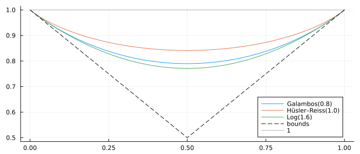

Sample scatter (uniform scale)

C = GalambosCopula(2, 1.0)
plot(C, title="Galambos copula sample")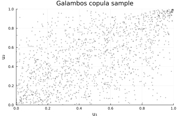

Conditional distortion (EV example)

C = HuslerReissCopula(2, 1.2)
u2 = 0.4
D = condition(C, 2, u2)
ts = range(0.0, 1.0; length=401)
plot(ts, cdf.(Ref(D), ts); xlabel="u", ylabel="H_{1|2}(u|u₂=0.4)",
     title="Conditional distortion for Hüsler–Reiss")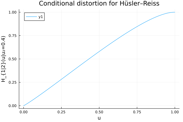

Rosenblatt sanity check (EV)

using StatsBase
U = rand(C, 2000)
S = reduce(hcat, (rosenblatt(C, U[:, i]) for i in 1:size(U,2)))
ts = range(0.0, 1.0; length=401)
EC = [ecdf(S[k, :]) for k in 1:2]
plot(ts, ts; label="Uniform", color=:blue, alpha=0.6, size=(650,300))
plot!(ts, EC[1].(ts); seriestype=:steppost, label="s₁", color=:black)
plot!(ts, EC[2].(ts); seriestype=:steppost, label="s₂", color=:gray)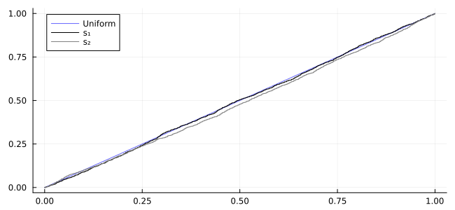

Available models

MTail

Copulas.MTail Type

MTail

Corresponds to the MCopula viewed as an etreme value copula.

source

NoTail

Copulas.NoTail Type

NoTail

Corresponds to the case where the pickads function is identically One, which means no particular tail behavior.

source

AsymGalambosTail

Copulas.AsymGalambosTail Type

AsymGalambosTail{T}, AsymGalambosCopula{T}

Fields:

• α::Real — dependence parameter

• θ₁::Real — asymmetry weight in [0,1]

• θ₂::Real — asymmetry weight in [0,1]

Constructor

AsymGalambosCopula(α, θ₁, θ₂)
ExtremeValueCopula(2, AsymGalambosTail(α, θ₁, θ₂))

The (bivariate) asymmetric Galambos extreme-value copula is parameterized by $\alpha \in [0,\mathrm{\infty })$ and ${\theta }_1,{\theta }_2\in [0,1]$. It is an EV copula with Pickands function

$$A(t)=1-(({\theta }_{1}t{)}^{-\alpha }+({\theta }_2(1-t){)}^{-\alpha }{)}^{-1/\alpha },t\in [0,1].$$

Special cases:

• α = 0 ⇒ IndependentCopula

• θ₁ = θ₂ = 0 ⇒ IndependentCopula

• θ₁ = θ₂ = 1 ⇒ GalambosCopula

References:

• [48] Families of min-stable multivariate exponential and multivariate extreme value distributions. Statist. Probab, 1990.

source

AsymLogTail

Copulas.AsymLogTail Type

AsymLogTail{T}, AsymLogCopula{T}

Fields:

• α::Real — dependence parameter (α ≥ 1)

• θ₁::Real — asymmetry weight in [0,1]

• θ₂::Real — asymmetry weight in [0,1]

Constructor

AsymLogCopula(α, θ₁, θ₂)
ExtremeValueCopula(2, AsymLogTail(α, θ₁, θ₂))

The (bivariate) asymmetric logistic extreme–value copula is parameterized by α ∈ [1, ∞) and θ₁, θ₂ ∈ [0,1]. Its Pickands dependence function is

$$A(t)=({\theta }_1^{\alpha }(1-t{)}^{\alpha }+{\theta }_2^{\alpha }{t}^{\alpha }{)}^{1/\alpha }+({\theta }_1-{\theta }_2)t+1-{\theta }_1,t\in [0,1].$$

Special cases:

• θ₁ = θ₂ = 1 ⇒ symmetric Logistic (Gumbel) copula

• θ₁ = θ₂ = 0 ⇒ independence (A(t) ≡ 1)

References:

• [49] : Tawn, Jonathan A. "Bivariate extreme value theory: models and estimation." Biometrika 75.3 (1988): 397-415.

source

AsymMixedTail

Copulas.AsymMixedTail Type

AsymMixedTail{T}, AsymMixedCopula{T}

Fields:

• θ₁::Real — parameter

• θ₂::Real — parameter

Constructor

AsymMixedCopula(θ₁, θ₂) ExtremeValueCopula(2, AsymMixedTail(θ₁, θ₂))

The (bivariate) asymmetric Mixed extreme-value copula is parameterized by two parameters ${\theta }_1$, ${\theta }_2$ subject to the following constraints:

• θ₁ ≥ 0

• θ₁ + θ₂ ≤ 1

• θ₁ + 2θ₂ ≤ 1

• θ₁ + 3θ₂ ≥ 0

Its Pickands dependence function is

$$A(t)={\theta }_2{t}^3+{\theta }_1{t}^2-({\theta }_1+{\theta }_2)t+1,t\in [0,1].$$

Special cases:

• θ₁ = θ₂ = 0 ⇒ IndependentCopula

• θ₂ = 0 ⇒ symmetric Mixed copula

References:

• [49] : Tawn, Jonathan A. "Bivariate extreme value theory: models and estimation." Biometrika 75.3 (1988): 397-415.

source

BC2Tail

Copulas.BC2Tail Type

BC2Tail{T}, BC2Copula{T}

Fields:

• a::Real — parameter (a ∈ [0,1])

• b::Real — parameter (b ∈ [0,1])

Constructor

BC2Copula(a, b)
ExtremeValueCopula(2, BC2Tail(a, b))

The bivariate BC2 extreme-value copula is parameterized by two parameters $a,b\in [0,1]$. Its Pickands dependence function is

$$A(t)=max\{at,b(1-t)\}+max\{(1-a)t,(1-b)(1-t)\},t\in [0,1].$$

References:

• [50] Mai, J. F., & Scherer, M. (2011). Bivariate extreme-value copulas with discrete Pickands dependence measure. Extremes, 14, 311-324. Springer, 2011.

source

CuadrasAugeTail

Copulas.CuadrasAugeTail Type

CuadrasAugeTail{T}, CuadrasAugeCopula{T}

Fields:

• θ::Real — dependence parameter, θ ∈ [0,1]

Constructor

CuadrasAugeCopula(θ)
ExtremeValueCopula(2, CuadrasAugeTail(θ))

The (bivariate) Cuadras-Augé extreme-value copula is parameterized by $\theta \in [0,1]$. Its Pickands dependence function is

$$A(t)=max\{t,1-t\}+(1-\theta )min\{t,1-t\},t\in [0,1].$$

Special cases:

• θ = 0 ⇒ IndependentCopula

• θ = 1 ⇒ MCopula (comonotone copula)

References:

• [51] Mai, J. F., & Scherer, M. (2012). Simulating copulas: stochastic models, sampling algorithms, and applications (Vol. 4). World Scientific.

source

GalambosTail

Copulas.GalambosTail Type

GalambosTail{T}, GalambosCopula{T}

Fields:

• θ::Real — dependence parameter, θ ≥ 0

Constructor

GalambosCopula(θ)
ExtremeValueCopula(2, GalambosTail(θ))

The (bivariate) Galambos extreme-value copula is parameterized by $\theta \in [0,\mathrm{\infty })$. Its Pickands dependence function is

$$A(t)=1-(t^{-\theta }+(1-t{)}^{-\theta }{)}^{-1/\theta },t\in (0,1).$$

Special cases:

• θ = 0 ⇒ IndependentCopula

• θ = ∞ ⇒ MCopula (upper Fréchet-Hoeffding bound)

References:

• [52] Galambos, J. (1975). Order statistics of samples from multivariate distributions. Journal of the American Statistical Association, 70(351a), 674-680.

source

HuslerReissTail

Copulas.HuslerReissTail Type

HuslerReissTail{T}, HuslerReissCopula{T}

Fields:

• θ::Real — dependence parameter, θ ≥ 0

Constructor

HuslerReissCopula(θ)
ExtremeValueCopula(2, HuslerReissTail(θ))

The (bivariate) Hüsler-Reiss extreme-value copula is parameterized by $\theta \in [0,\mathrm{\infty })$. Its Pickands dependence function is

$$A(t)=t\mathrm{\Phi }({\theta }^{-1}+\frac{1}{2}\theta \log (\frac{t}{1-t}))+(1-t)\mathrm{\Phi }({\theta }^{-1}+\frac{1}{2}\theta \log (\frac{1-t}{t}))$$

where $\mathrm{\Phi }$ is the standard normal cdf.

Special cases:

• θ = 0 ⇒ IndependentCopula

• θ = ∞ ⇒ MCopula (upper Fréchet-Hoeffding bound)

References:

• [53] Hüsler, J., & Reiss, R. D. (1989). Maxima of normal random vectors: between independence and complete dependence. Statistics & Probability Letters, 7(4), 283-286.

source

LogTail

Copulas.LogTail Type

LogTail{T}, LogCopula{T}

Fields:

• θ::Real — dependence parameter, θ ∈ [0,1]

Constructor

LogCopula(θ)
ExtremeValueCopula(2, LogTail(θ))

The (bivariate) Mixed extreme-value copula is parameterized by $\theta \in [0,1]$. Its Pickands dependence function is

$$A(t)=\theta t^2-\theta t+1,t\in [0,1].$$

Special cases:

• θ = 0 ⇒ IndependentCopula

References:

• [49] : Tawn, Jonathan A. "Bivariate extreme value theory: models and estimation." Biometrika 75.3 (1988): 397-415.

source

MixedTail

Copulas.MixedTail Type

MixedTail{T}, MixedCopula{T}

Fields:

• θ::Real — dependence parameter, θ ∈ [0,1]

Constructor

MixedCopula(θ)
ExtremeValueCopula(2, MixedTail(θ))

The (bivariate) Mixed extreme-value copula is parameterized by $\theta \in [0,1]$. Its Pickands dependence function is

$$A(t)=\theta t^2-\theta t+1,t\in [0,1].$$

Special cases:

• θ = 0 ⇒ IndependentCopula

References:

• [49] : Tawn, Jonathan A. "Bivariate extreme value theory: models and estimation." Biometrika 75.3 (1988): 397-415.

source

MOTail

Copulas.MOTail Type

MOTail{T}, MOCopula{T}

Fields:

• λ₁::Real — parameter ≥ 0

• λ₂::Real — parameter ≥ 0

• λ₁₂::Real — parameter ≥ 0

Constructor

MOCopula(λ₁, λ₂, λ₁₂)
ExtremeValueCopula(2, MOTail(λ₁, λ₂, λ₁₂))

The (bivariate) Marshall-Olkin extreme-value copula is parameterized by ${\lambda }_i\in [0,\mathrm{\infty }),i=1,2,\{1,2\}$ Its Pickands dependence function is

$$A(t)=\frac{{\lambda }_1(1-t)}{{\lambda }_1+{\lambda }_{1,2}}+\frac{{\lambda }_{2}t}{{\lambda }_2+{\lambda }_{1,2}}+{\lambda }_{1,2}max\{\frac{1-t}{{\lambda }_1+{\lambda }_{1,2}},\frac{t}{{\lambda }_2+{\lambda }_{1,2}}\}$$

Special cases:

• If λ₁₂ = 0, reduces to an asymmetric independence-like form.

• If λ₁ = λ₂ = 0, degenerates to complete dependence.

References:

• [51] Mai, J. F., & Scherer, M. (2012). Simulating copulas: stochastic models, sampling algorithms, and applications (Vol. 4). World Scientific.

source

tEVTail

Copulas.tEVTail Type

tEVTail{Tdf,Tρ}, tEVCopula{T}

Fields:

• ν::Real — degrees of freedom (ν > 0)

• ρ::Real — correlation parameter (ρ ∈ (-1,1])

Constructor

tEVCopula(ν, ρ)
ExtremeValueCopula(2, tEVTail(ν, ρ))

The (bivariate) extreme-t copula is parameterized by $\nu >0$ and \rho \in (-1,1]``. Its Pickands dependence function is

$$A(x)=x{t}_{\nu +1}(Z_x)+(1-x)t_{\nu +1}(Z_{1-x})$$

Where $t_{\nu +1}$ is the cumulative distribution function (CDF) of the standard t distribution with $\nu +1$ degrees of freedom and

$$Z_x=\sqrt{\frac{1+\nu }{1-{\rho }^2}}({\left(\frac{x}{1-x}\right)}^{1/\nu }-\rho )$$

Special cases:

• ρ = 0 ⇒ IndependentCopula

• ρ = 1 ⇒ M Copula (upper Fréchet-Hoeffding bound)

References:

• [54] Nikoloulopoulos, A. K., Joe, H., & Li, H. (2009). Extreme value properties of multivariate t copulas. Extremes, 12, 129-148.

source

EmpiricalEVTail

Copulas.EmpiricalEVTail Type

EmpiricalEVTail, EmpiricalEVCopula

Fields:

• tgrid::Vector{Float64} — evaluation grid in (0,1)

• Ahat::Vector{Float64} — estimated Pickands function values on tgrid

• slope::Vector{Float64} — per-segment slopes for linear interpolation

Constructor

EmpiricalEVTail(u; method=:ols, grid=401, eps=1e-3, pseudo_values=true) ExtremeValueCopula(2, EmpiricalEVTail(u; ...))

The empirical extreme-value (EV) copula (bivariate) is defined from pseudo-observations u = (U₁, U₂) and a nonparametric estimator of the Pickands dependence function. Supported estimators are:

• :pickands — classical Pickands estimator

• :cfg — Capéraà–Fougères–Genest (CFG) estimator

• :ols — OLS-intercept estimator

For stability, the estimated function is always projected onto the class of valid Pickands functions (convex, bounded between max(t,1-t) and 1, with endpoints fixed at 1).

Its Pickands function is

Â(t),  t ∈ (0,1),

evaluated via piecewise linear interpolation on the grid tgrid.

References

• [caperaa1997nonparametric] Capéraà, Fougères, Genest (1997) Biometrika

• [gudendorf2011nonparametric] Gudendorf, Segers (2011) Journal of Multivariate Analysis

source

References

1. H. Joe. Dependence Modeling with Copulas (CRC press, 2014).

2. G. Gudendorf and J. Segers. Extreme-value copulas. In: Copula Theory and Its Applications: Proceedings of the Workshop Held in Warsaw, 25-26 September 2009 (Springer, 2010); pp. 127–145.

3. K. Ghoudi, A. Khoudraji and E. L.-P. Rivest. Propriétés statistiques des copules de valeurs extrêmes bidimensionnelles. Canadian Journal of Statistics 26, 187–197 (1998).

4. P. Deheuvels. On the limiting behavior of the Pickands estimator for bivariate extreme-value distributions. Statistics & Probability Letters 12, 429–439 (1991).

5. J.-F. Mai and M. Scherer. Financial engineering with copulas explained (Springer, 2014).

6. H. Joe. Families of min-stable multivariate exponential and multivariate extreme value distributions. Statistics & probability letters 9, 75–81 (1990).

7. J. A. Tawn. Bivariate extreme value theory: models and estimation. Biometrika 75, 397–415 (1988).

8. J.-F. Mai and M. Scherer. Bivariate extreme-value copulas with discrete Pickands dependence measure. Extremes 14, 311–324 (2011).

9. J.-F. Mai and M. Scherer. Simulating copulas: stochastic models, sampling algorithms, and applications. Vol. 4 (World Scientific, 2012).

10. J. Galambos. Order statistics of samples from multivariate distributions. Journal of the American Statistical Association 70, 674–680 (1975).

11. J. Hüsler and R.-D. Reiss. Maxima of normal random vectors: between independence and complete dependence. Statistics & Probability Letters 7, 283–286 (1989).

12. A. K. Nikoloulopoulos, H. Joe and H. Li. Extreme value properties of multivariate t copulas. Extremes 12, 129–148 (2009).